-
MCP Tool Explorer Supports MCP Apps: Protocol, Code, and the Fine Print
MCP Apps adds interactive HTML UIs to MCP tools. This post covers the protocol, the host implementation, and the sandbox constraints that only show up when you actually build it.
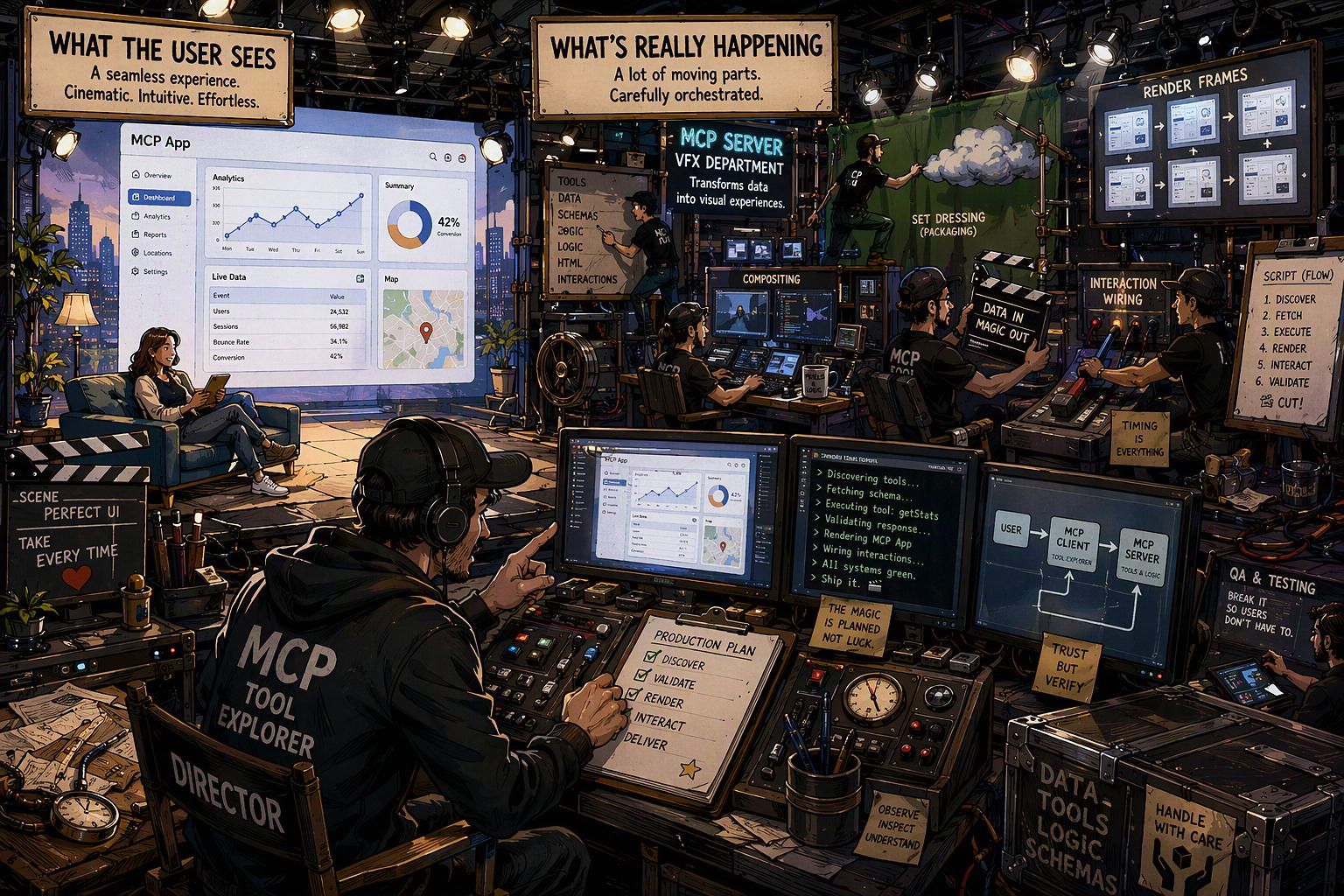
MCP Tool Explorer is a VS Code extension for exploring MCP servers: browsing tools, resources, and prompts, calling them, and inspecting results. With this update it also renders MCP App UIs inline, next to the regular result view.
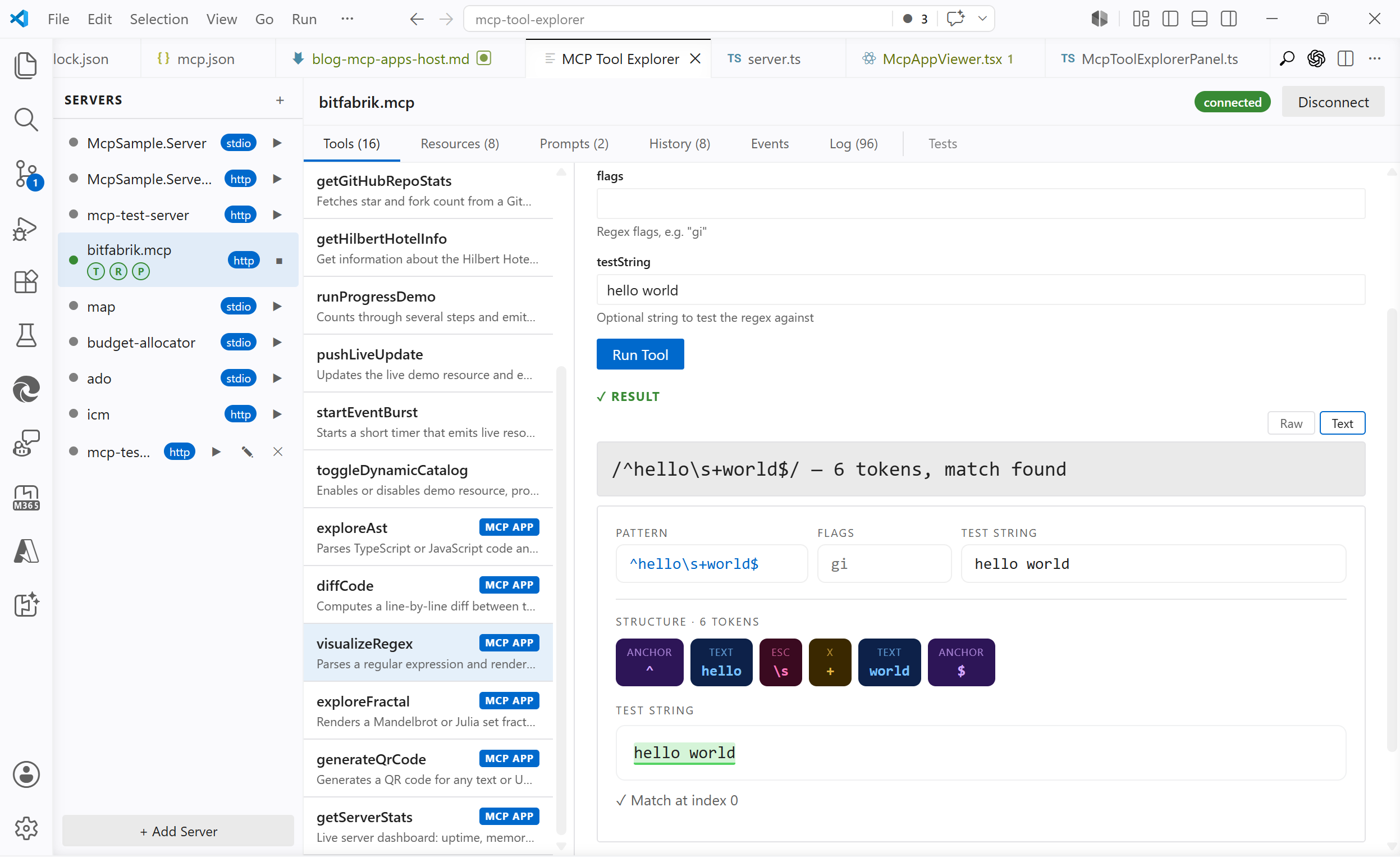
A few examples running inside the extension: one from the official SDK sample, five built as test cases.
budget-allocator (official SDK sample)
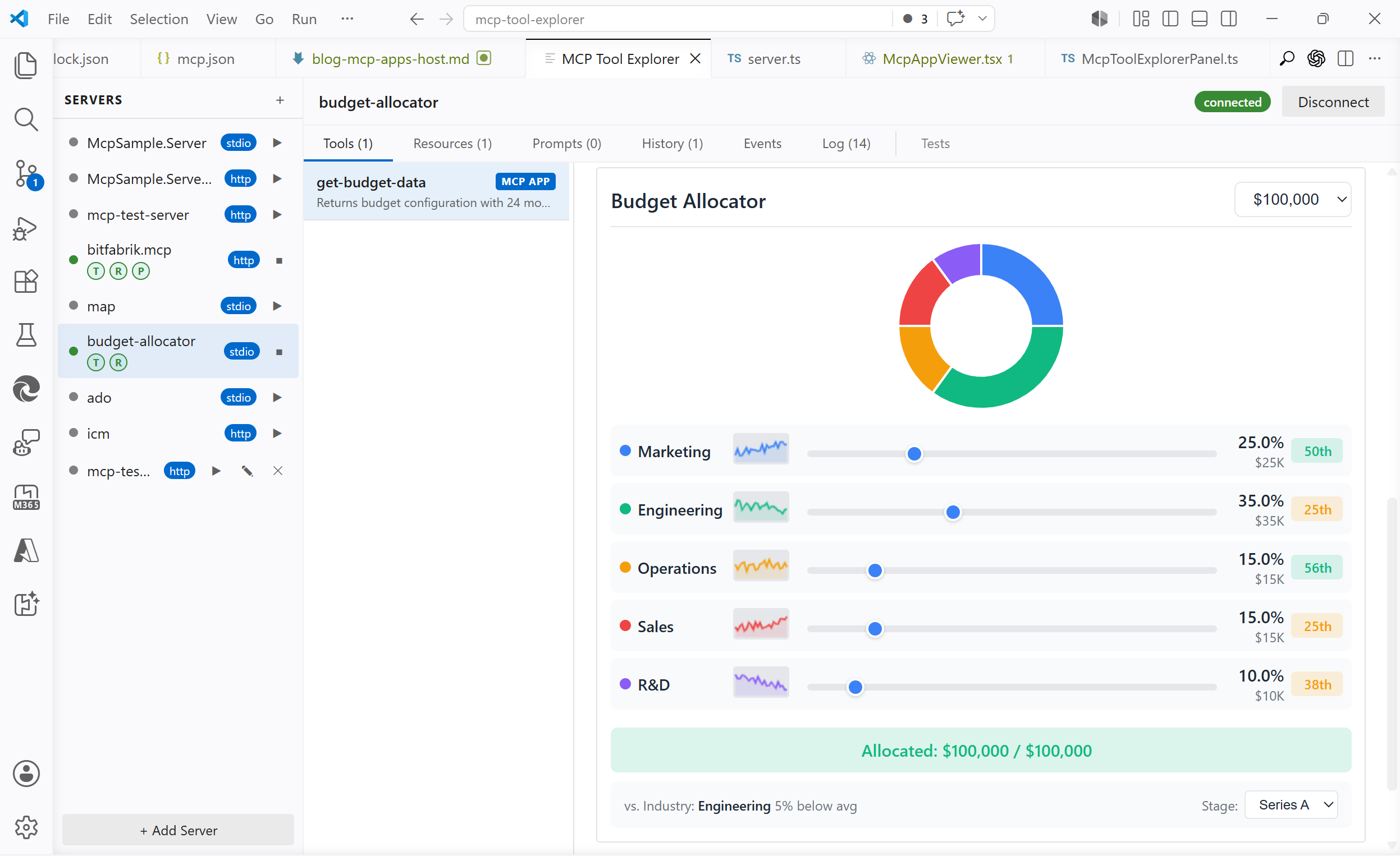
mcp.json"budget-allocator": { "command": "npx", "args": ["-y", "@modelcontextprotocol/server-budget-allocator", "--stdio"] },Regex visualizer: parses a regex and renders an interactive token breakdown with optional match highlighting
 on
on https://bitfabrik.io/mcpQR code generator: generates a QR code for any text or URL, live-updating as you type
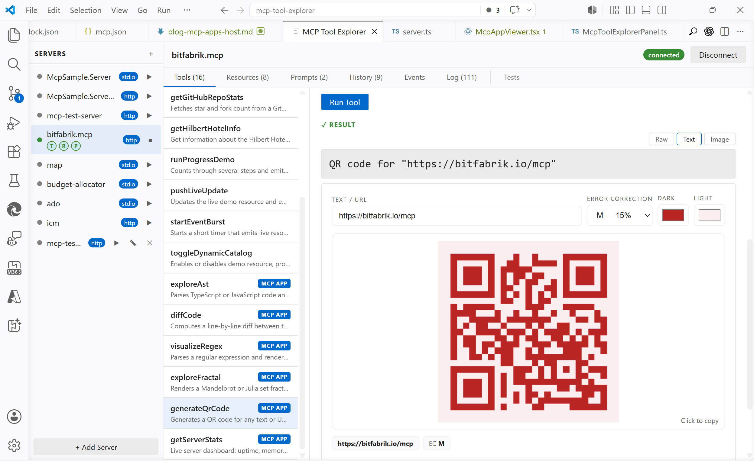 on
on https://bitfabrik.io/mcpCode diff viewer: computes a line-by-line diff and renders a visual unified diff with syntax highlighting
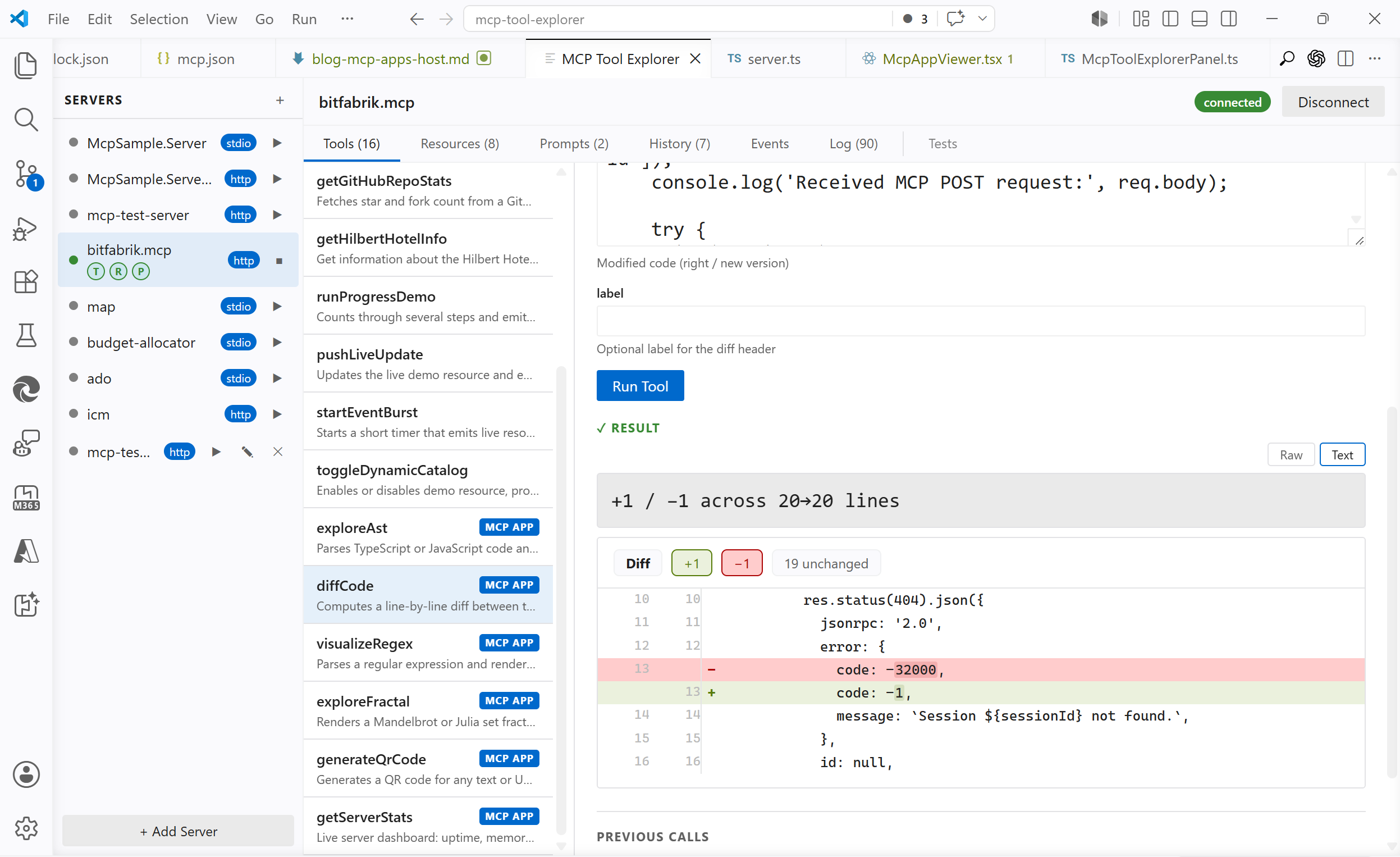 on
on https://bitfabrik.io/mcpFractal explorer: renders a Mandelbrot or Julia set; click to zoom
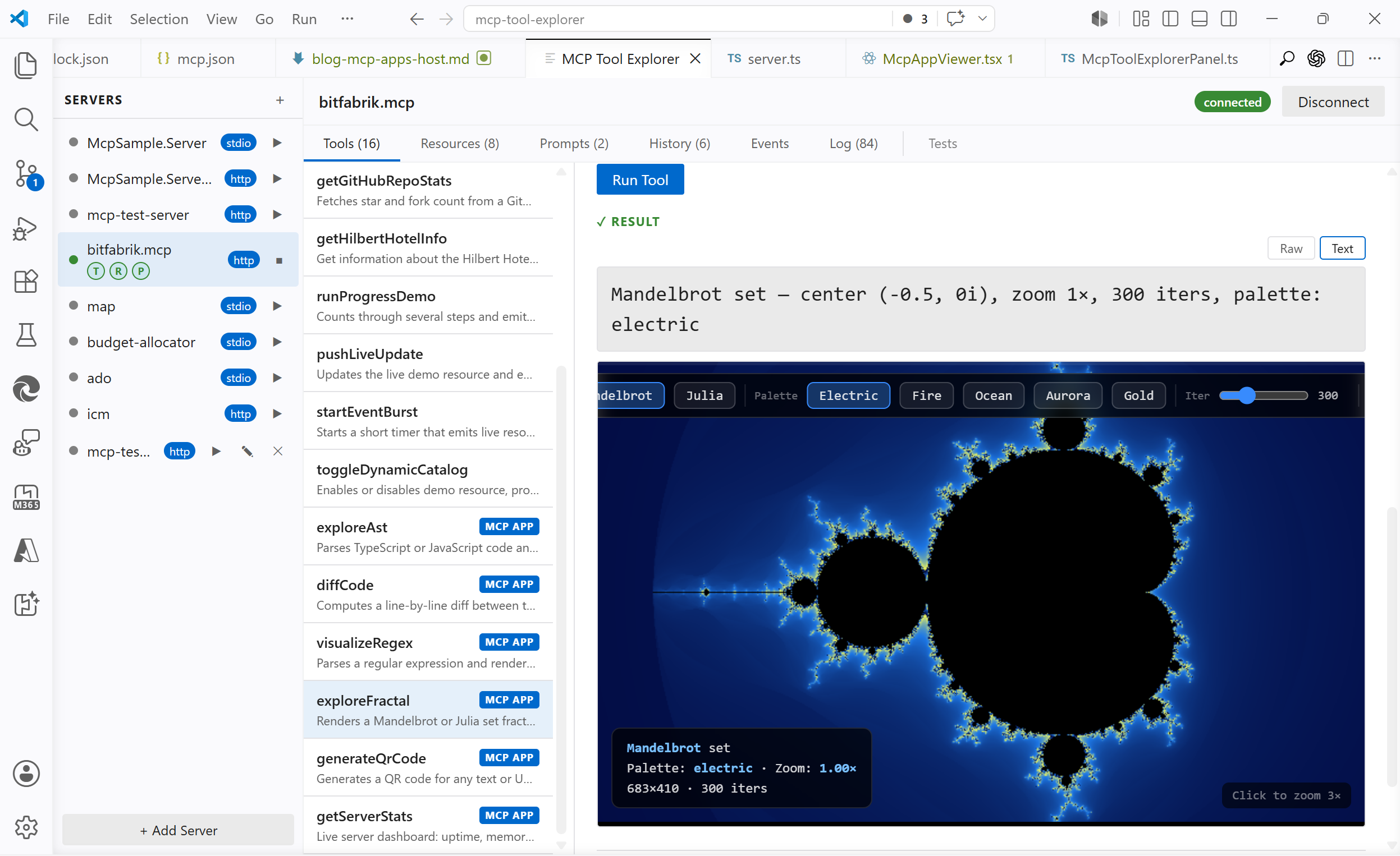 on
on https://bitfabrik.io/mcpServer stats dashboard: live view of uptime, call counts, and recent requests
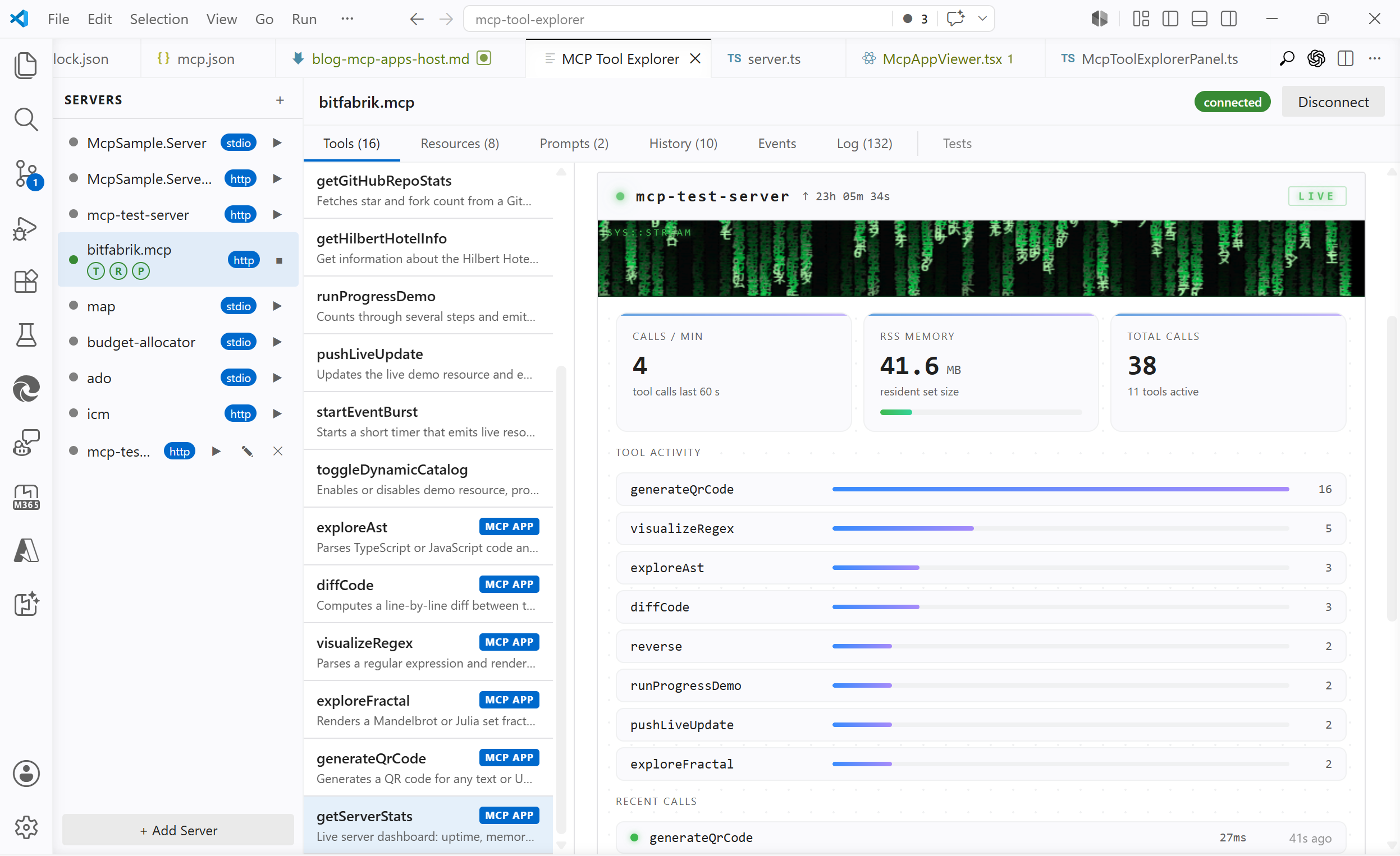 on
on https://bitfabrik.io/mcpWhat MCP Apps Actually Is
MCP tools normally return text or JSON. MCP Apps extends MCP: a tool can include a
ui://resource URI in its_metafield. The host fetches that URI, gets back a full HTML document, renders it in a sandboxed iframe, and proxies JSON-RPC 2.0 messages between the iframe and the MCP server viapostMessage.That is the whole mechanism. The protocol is not exotic; it reuses the existing MCP
resources/readcall for the HTML fetch and standard JSON-RPC 2.0 for the iframe bridge. The spec explicitly notes that you do not need an SDK to implement it.Supported hosts as of today: Claude, ChatGPT, VS Code, Goose, Postman, MCPJam.
The Architecture
The moving parts:
+------------------------------------------------------------+
|  VS Code                                                   |
|                                                            |
|  +------------------------------+                          |
|  |  Extension Host (Node.js)    |                          |
|  |  McpToolExplorerPanel.ts     |---------- HTTP ----------> MCP Server
|  |  McpClientManager.ts         |      (localhost:3000)    | (server.ts)
|  +------------------------------+                          |
|              |  postMessage                                |
|  +-----------v------------------+                          |
|  |  Webview (Chromium)          |                          |
|  |  McpAppViewer.tsx (React)    |                          |
|  |  +--------------------------+|                          |
|  |  | iframe (sandboxed)       ||                          |
|  |  | MCP App HTML             ||                          |
|  |  | (postMessage only,       ||                          |
|  |  |  no network access)      ||                          |
|  |  +--------------------------+|                          |
|  +------------------------------+                          |
+------------------------------------------------------------+
The iframe has
sandbox="allow-scripts"and nothing else: noallow-same-origin, no network access, no cookies, nolocalStorage.McpAppVieweris the sole intermediary: it catchespostMessagefrom the iframe and routes everything through the extension host to the real MCP server over HTTP.One thing that is not obvious from the spec: the bridge lives in the webview, not inside the iframe. The app sends messages to
window.parent; the host catches them from the outside. Nothing is injected into the iframe.The Protocol
A tool advertises its UI in
_meta:{ "name": "generateQrCode", "_meta": { "ui": { "resourceUri": "ui://mcp-test-server/qr-code" } } }The host signals support during
initialize:new Client( { name: 'my-host', version: '1.0.0' }, { capabilities: { extensions: { 'io.modelcontextprotocol/ui': { mimeTypes: ['text/html;profile=mcp-app'] }, }, }, } )After a tool call, if the result's tool definition has
_meta.ui.resourceUri, the host callsresources/readon that URI, gets HTML back incontent[0].text, and hands it to the webview. The iframe then runs the full MCP handshake sequence overpostMessage:iframe → Host: initialize Host → iframe: initialize result iframe → Host: notifications/initialized iframe → Host: ui/initialize (MCP Apps extension handshake) Host → iframe: ui/initialize result (includes hostContext: theme, platform, displayMode) iframe → Host: ui/notifications/initialized ← "I am ready" Host → iframe: ui/notifications/tool-input { arguments: { ... } } Host → iframe: ui/notifications/tool-result { content: [...], structuredContent: { ... } }After that, the iframe can call
tools/callandresources/readinteractively, and sendsui/notifications/size-changedto drive iframe resizing.Implementing the Host
Advertising capability and fetching the HTML
The capability is declared in the
Clientconstructor (shown above). On the server side, attaching_meta.uito a tool registration requires a// @ts-ignorefor now: the field is protocol-level but not yet in the SDK TypeScript types:Without SDK:
// @ts-ignore — _meta is not yet typed in @modelcontextprotocol/sdk
server.registerTool('generateQrCode', {
  title: 'QR Code Generator',
  description: 'Generates a QR code for any text or URL',
  inputSchema: { text: z.string().describe('Text or URL to encode') },
  _meta: { ui: { resourceUri: 'ui://mcp-test-server/qr-code' } },
}, handler);
With SDK (
@modelcontextprotocol/ext-apps/server),getUiCapabilitychecks whether the connecting host supports UI before_metais attached:import { getUiCapability, RESOURCE_MIME_TYPE } from "@modelcontextprotocol/ext-apps/server"; const uiCap = getUiCapability(clientCapabilities); if (uiCap?.mimeTypes?.includes(RESOURCE_MIME_TYPE)) { tool._meta = { ui: { resourceUri: 'ui://mcp-test-server/qr-code' } }; }When a tool result arrives, the host reads the HTML and builds the CSP before handing it to the webview:
case 'fetchUiResource': {
  const result = await this._clientManager.readResource(message.serverId, message.uri);
  const content = result.contents?.[0];
  const html = content && 'text' in content && typeof content.text === 'string'
    ? content.text : undefined;
  if (!html) { /* send error */ break; }
  const uiMeta = (content as any)?._meta?.ui;
  this._post({ type: 'uiResourceContent', requestId: message.requestId, html, csp: uiMeta?.csp });
  break;
}
The
_meta.ui.cspfield is optional. If the server declares external domains there (CDN hosts for scripts, API endpoints), the host adds them to the iframe's CSP. Without it,default-src 'none'applies and all external fetches are blocked. That is by design.function buildCsp(csp: CspMeta | undefined): string { const connect = csp?.connectDomains?.join(' ') ?? ''; const resources = csp?.resourceDomains?.join(' ') ?? ''; return [ "default-src 'none'", `script-src 'self' 'unsafe-inline' ${resources}`.trimEnd(), `connect-src 'self' ${connect}`.trimEnd(), // … ].join('; '); }The CSP is injected as a
tag prepended to the HTML before writing it toiframe.srcdoc. The iframe is shown immediately when the HTML arrives, not after the MCP handshake inside the iframe completes. Gating on that internal handshake would leave the host stuck on "Loading…" if the app is slow or broken.The JSON-RPC bridge
The
@modelcontextprotocol/ext-apps/app-bridgepackage wraps the whole handshake in a few lines:import { AppBridge } from '@modelcontextprotocol/ext-apps/app-bridge'; const bridge = new AppBridge(iframeElement, mcpClient); bridge.onReady(() => { bridge.sendToolInput({ arguments: toolArgs }); bridge.sendToolResult(result); });For a VS Code webview with its own React architecture, a vanilla implementation was the more practical choice: the webview already has its own message bus between extension host and UI, and adding a second one creates more complexity than it removes. The whole bridge is around 150 lines. It handles
initialize,ui/initialize,tools/call,resources/read,ui/open-link,ui/notifications/size-changed, andping. Each message type is explicit, which is useful while the protocol is still maturing.One detail that the sequence diagram makes clear:
structuredContentmust survive the entire round-trip. It is a first-class field added in MCP spec 2026-01-26; it sits alongside the plaincontentarray and carries the machine-readable data that drives the app's UI. If any layer in the pipeline silently drops it, the iframe renders its empty state:// host → webview → McpAppViewer props → ui/notifications/tool-result if (m.type === 'toolResult') { sendToIframe({ jsonrpc: '2.0', id, result: { content: m.result, isError: m.isError, ...(m.structuredContent !== undefined ? { structuredContent: m.structuredContent } : {}), }}); }Dynamic height
The iframe cannot read its own
scrollHeightwithoutallow-same-origin. Instead, the app sendsui/notifications/size-changedwith its rendered height and the host resizes the iframe element accordingly:<iframe ref={iframeRef} sandbox="allow-scripts" srcdoc={preparedHtml} style={{ height: iframeHeight }} title="MCP App" />Startup Sequence
User clicks "Run"
       |
       v
ToolsPanel calls Extension
Extension calls MCP Server ──────────────────────────── HTTP POST
                            <────────── structuredContent ───────

McpAppViewer mounts, sends fetchUiResource
Extension calls resources/read("ui://…") ──────────── HTTP GET
                                          <──── HTML ────────────
iframe.srcdoc = html   ←── iframe starts

iframe                     McpAppViewer
  |── initialize ─────────────────────>|
  |<── result (ok) ────────────────────|
  |── ui/initialize ──────────────────>|
  |<── result (theme, platform, …) ────|
  |── ui/notifications/initialized ───>|
  |<── tool-input  { arguments }  ─────|   ← original args
  |<── tool-result { structuredContent}|   ← original result
  |
  renders initial state
Interactive tool calls afterward go through the same proxy path:
iframe → postMessage → McpAppViewer → extension host → HTTP → MCP server → back.Building an App: The QR Code Example
The QR code generator was built without a framework: plain JavaScript, JSON-RPC 2.0 over
postMessage. It exposed two sandbox constraints immediately.SVG data URIs are blocked.
QRCode.toString(text, { type: 'svg' })returns an SVG string. Putting it in an
// ✗ blocked img.src = 'data:image/svg+xml,' + encodeURIComponent(svg); // ✓ works fine in sandboxed iframes const pngDataUrl = await QRCode.toDataURL(text, { width: 300 }); img.src = pngDataUrl;navigator.clipboardis silently unavailable. The null origin has no clipboard permission. The fallback that still works:// ✗ silently fails await navigator.clipboard.writeText(text); // ✓ works even in sandboxed null origin const ta = document.createElement('textarea'); ta.value = text; document.body.appendChild(ta); ta.select(); document.execCommand('copy'); document.body.removeChild(ta);The app-side handshake is straightforward. The SDK's React binding handles it automatically; without it:
async function init() {
  await request('initialize', {
    protocolVersion: '2026-01-26',
    capabilities: {},
    clientInfo: { name: 'qr-code-app', version: '1.0.0' },
  });
  notify('notifications/initialized');

  const uiRes = await request('ui/initialize', {
    protocolVersion: '2026-01-26',
    clientInfo: { name: 'qr-code-app', version: '1.0.0' },
  });
  // uiRes.hostContext.theme → 'dark' | 'light'

  notify('ui/notifications/initialized');
  // host now sends tool-input and tool-result
}
Host Implementation Reference
Capability Advertise extensions['io.modelcontextprotocol/ui']ininitializeHTML fetch Standard resources/readon theui://URISandbox allow-scriptsonly, noallow-same-origin, noallow-top-navigationCSP Build from _meta.ui.csp;default-src 'none'as baselineBridge Handle postMessagefrom the webview side; nothing injected into the iframestructuredContentMCP spec 2026-01-26; thread it through every layer of the pipeline Timing Show the iframe when HTML arrives, not when the SDK handshake completes Resize Handle ui/notifications/size-changedto drive iframe heightTheme Pass hostContext.themeinui/initializeresultCDN scripts Only if server declares the domain in _meta.ui.csp.resourceDomainsObservations
The protocol is simpler than it first appears. Once the architecture is clear (iframe sends to
window.parent, webview catches from outside, extension host proxies over HTTP), the rest is just message routing. The non-obvious parts are the sandbox constraints (eval, SVG data URIs, clipboard all blocked withoutallow-same-origin) and the requirement to carrystructuredContentthrough every layer. Both are easy to miss until something silently fails.The SDK and the vanilla path produce the same result. The SDK is more concise on the app side; the vanilla implementation makes every protocol message explicit, which is useful when the spec is still evolving.
MCP Tool Explorer is available in the VS Code Marketplace. Point it at any MCP server that implements the spec; the UI appears automatically alongside the regular result view.
-
Kirschstreusel 🍒🥧
Sonntag. Ein Ablauf, der sich nicht anmeldet.
Der Ofen ist schon auf Temperatur, bevor überhaupt entschieden ist, ob das Ergebnis dokumentiert werden soll. Der Kirschstreusel ist zu diesem Zeitpunkt noch eher ein Versprechen. Die Oberfläche unfertig, die Struktur noch im Übergang. Die Hitze beginnt langsam Ordnung zu schaffen.
Währenddessen passiert etwas, das sich so nicht wiederholen lässt. Die Streusel verändern ihre Farbe nur wenig, von trocken zu goldbraun, mit diesem kurzen Punkt davor, an dem die Textur kippen würde. Messen kann man den Moment nicht wirklich. Man erkennt ihn eher.
1/250s f/2,8 ISO 3200/36° 16-50mm f/2,8 VR f=31mm/47mm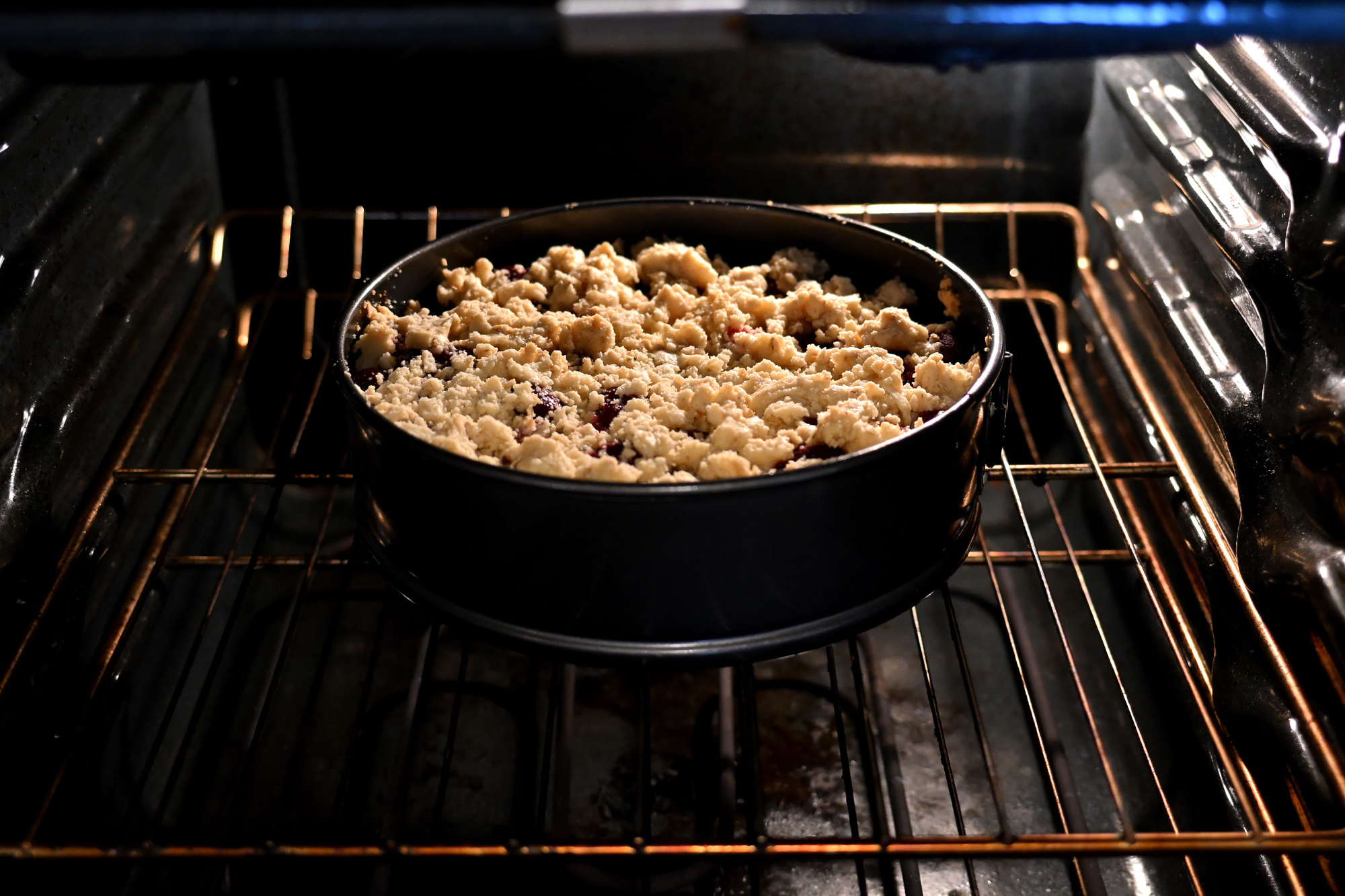
Danach kommt die Phase, in der alles noch zusammenhält. Der Kuchen bleibt in der Form, als müsste er selbst kurz prüfen, ob er stabil genug ist, um als Objekt zu existieren. Die Kirschen haben dabei ihre eigene Dynamik. Was vorher locker geschichtet war, ist jetzt gebunden, aber nicht starr. Oberfläche und Inneres passen langsam zusammen.
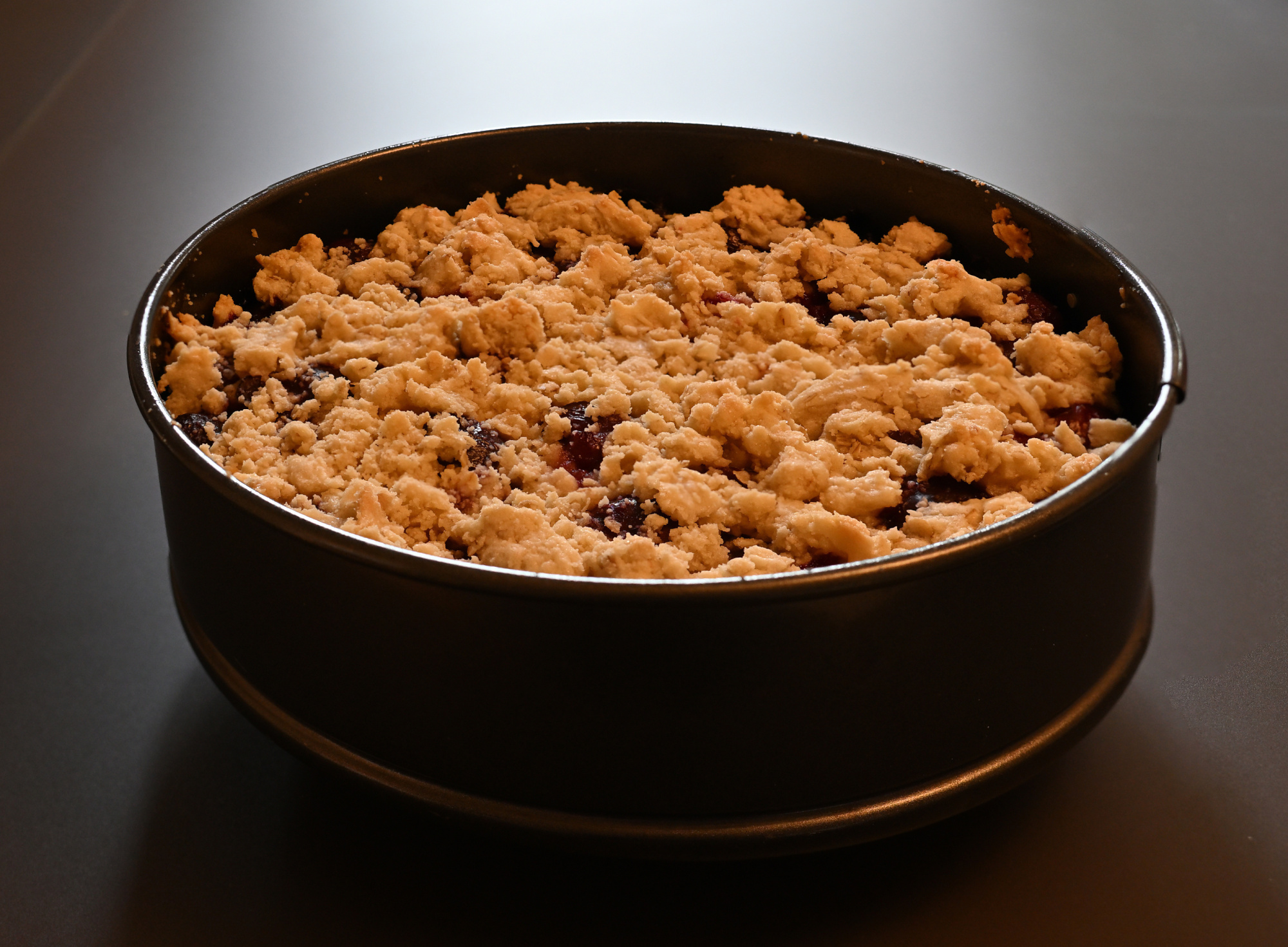
Erstellt mit Focus stacking
1/50s f/5 ISO 1000/31° 16-50mm f/2,8 VR f=33mm/49mm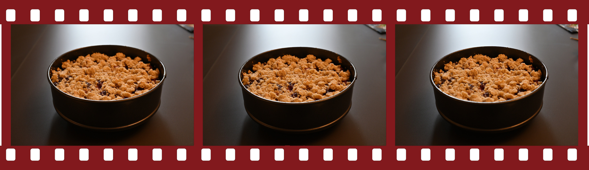
Auf dem Teller ist es wieder ein Übergangszustand. Abkühlen klingt passiv, ist es aber nicht. Dampf verschwindet, die Struktur zieht sich minimal zurück, Spannungen lösen sich. Die Oberfläche verliert etwas Glanz und gewinnt dafür an Klarheit. Ein kurzer Moment, in dem sich entscheidet, ob etwas als Bild bestehen bleibt oder nur als Erinnerung.
Erst mit dem ersten Schnitt wird es eindeutig. Die innere Struktur wird sichtbar. Schichtung, Verteilung, kleine Unregelmäßigkeiten, die vorher unsichtbar waren. Keine perfekte Geometrie, aber eine, die funktioniert.
und nimmt sich einen moment zeit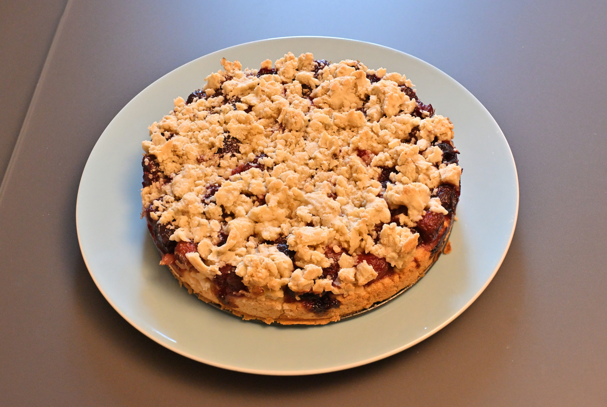
Das auch mit Focus stacking
1/50s f/5 ISO 1000/31° 16-50mm f/2,8 VR f=33mm/49mm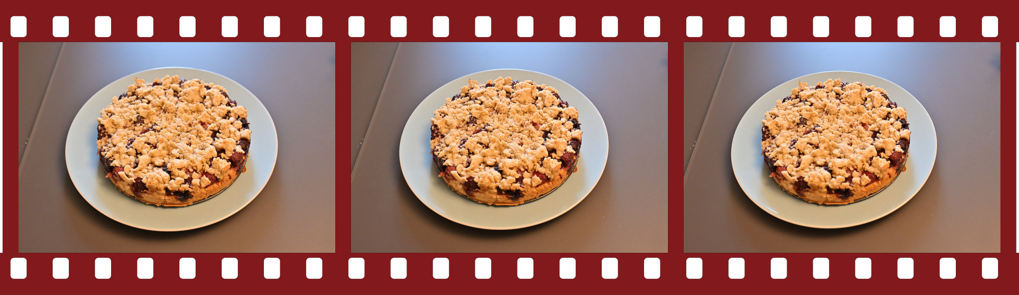
und wartet kurz bevor es weitergeht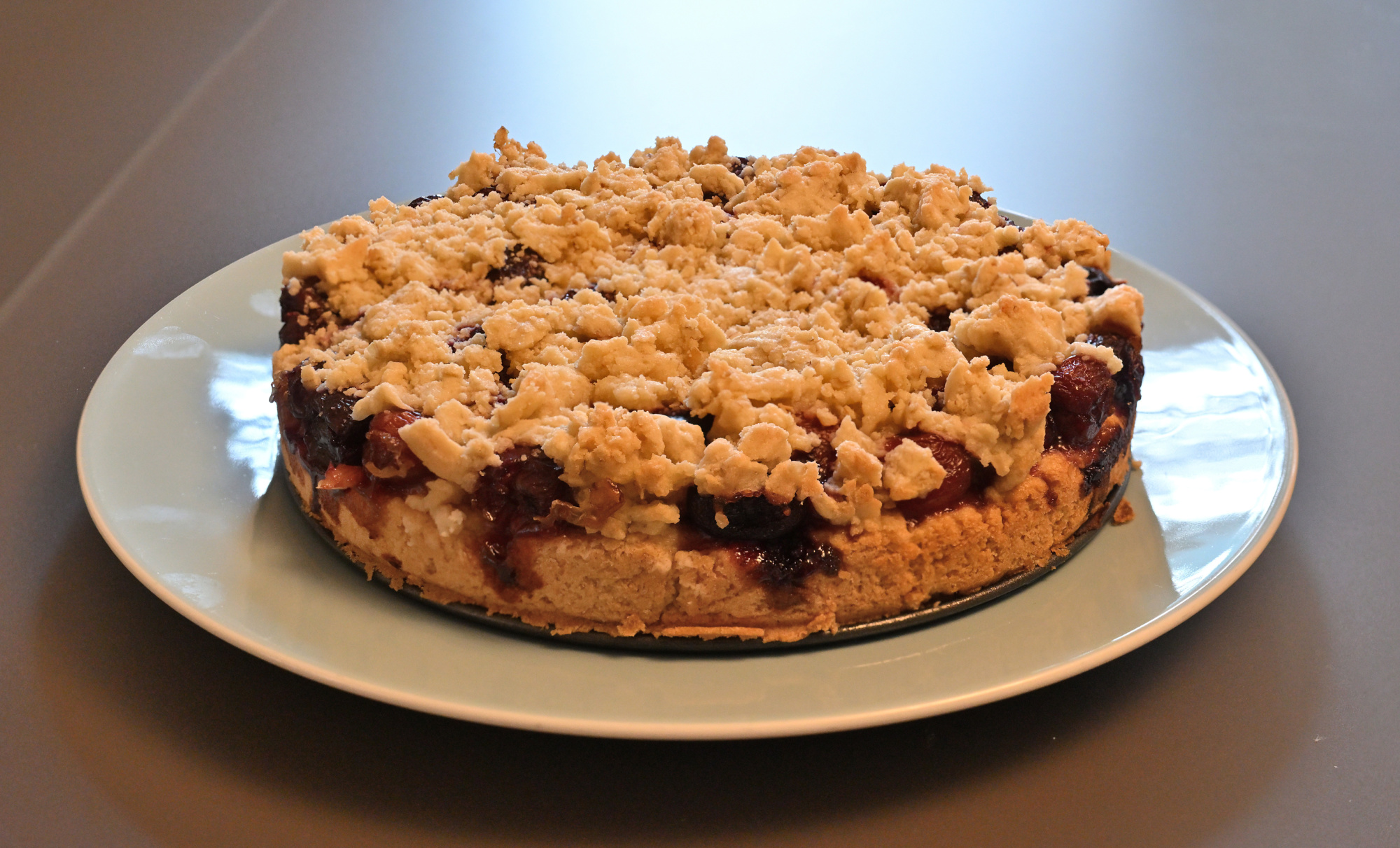
Und das auch
1/50s f/5 ISO 1000/31° 16-50mm f/2,8 VR f=33mm/49mm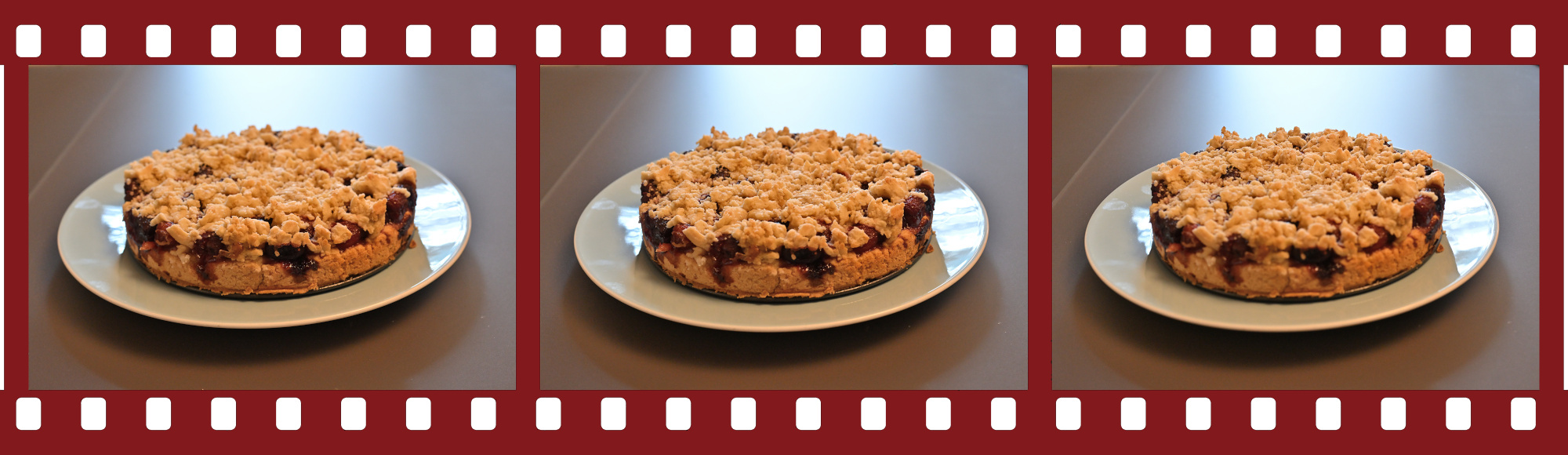
und passt jetzt schon fast vollständig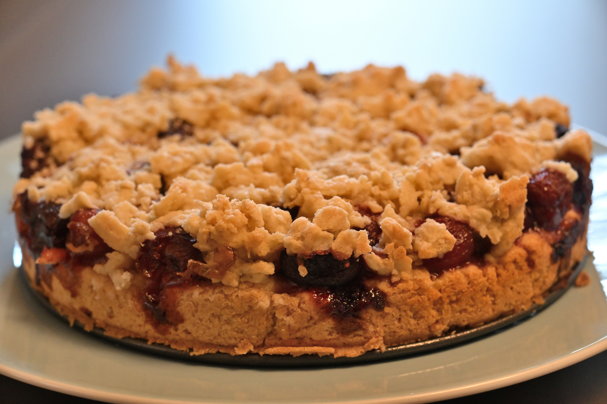
und übernimmt jetzt einfach1
1/100s f/2,8 ISO 100/21° 16-50mm f/2,8 VR f=41mm/61mm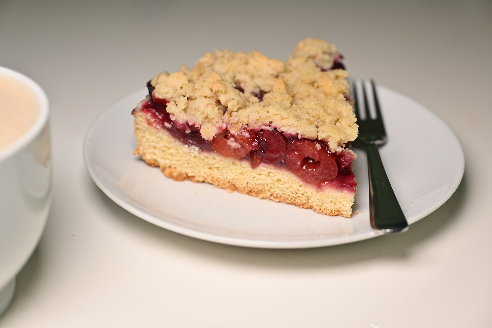
Kaffee trifft Kuchen ohne große Planung. Das Stück ist noch leicht warm, der Kaffee etwas zu heiß, aber das gleicht sich schnell aus. Man probiert kurz, schaut hin, und es passt. Auf dem Teller liegt noch ein zweites Stück. Erst einfach nur da, dann doch angeschnitten.
Für einen besonderen Sonntag genau richtig. Es bleibt eben nicht bei einem Stück.
-
Der Kuchen war diesmal pünktlich beim Shooting. Die Maske saß nicht immer, und bei der Pose gab es offenbar mehrere Meinungen.
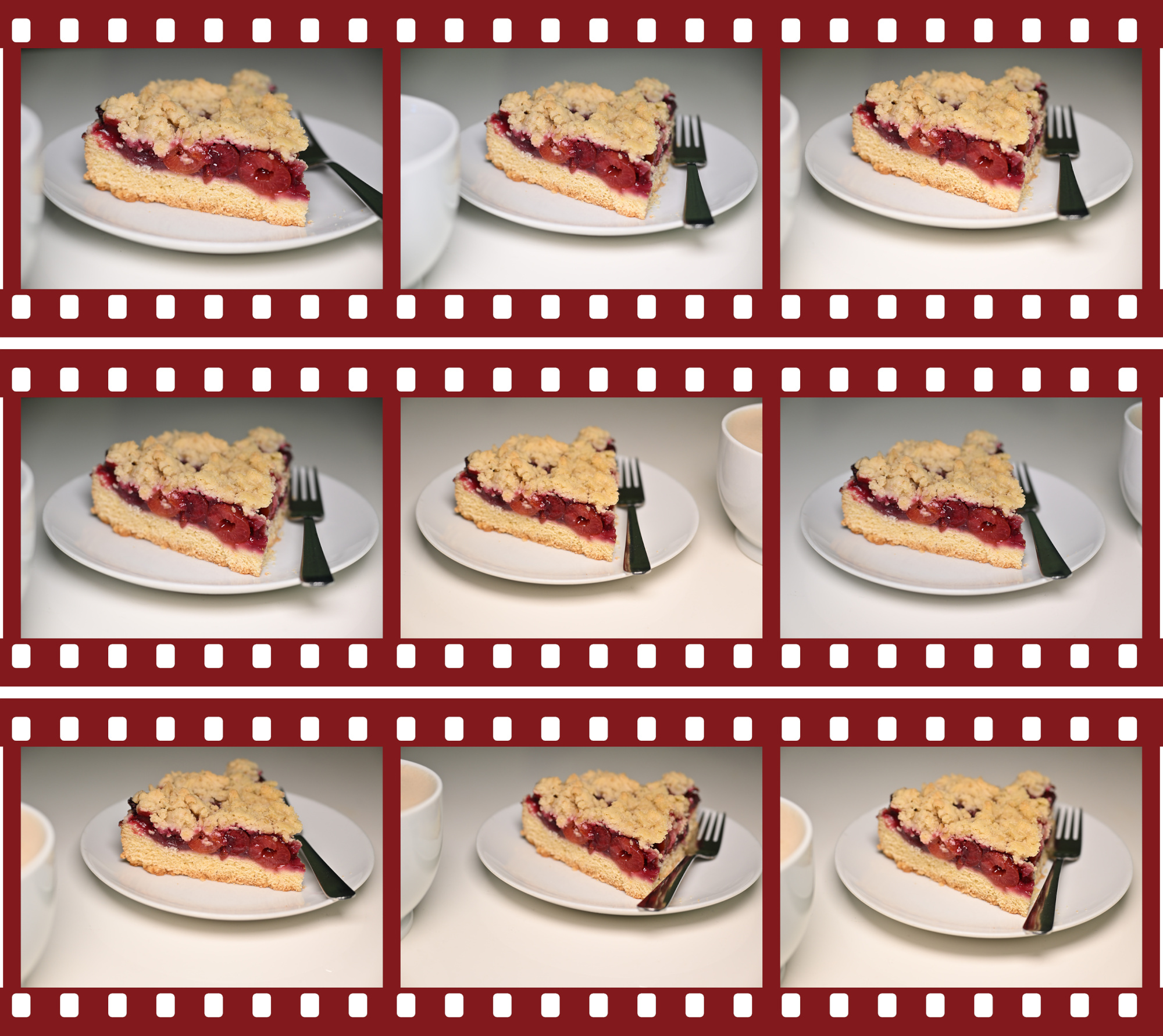
↩
-
-
When Focus Follows the Subject
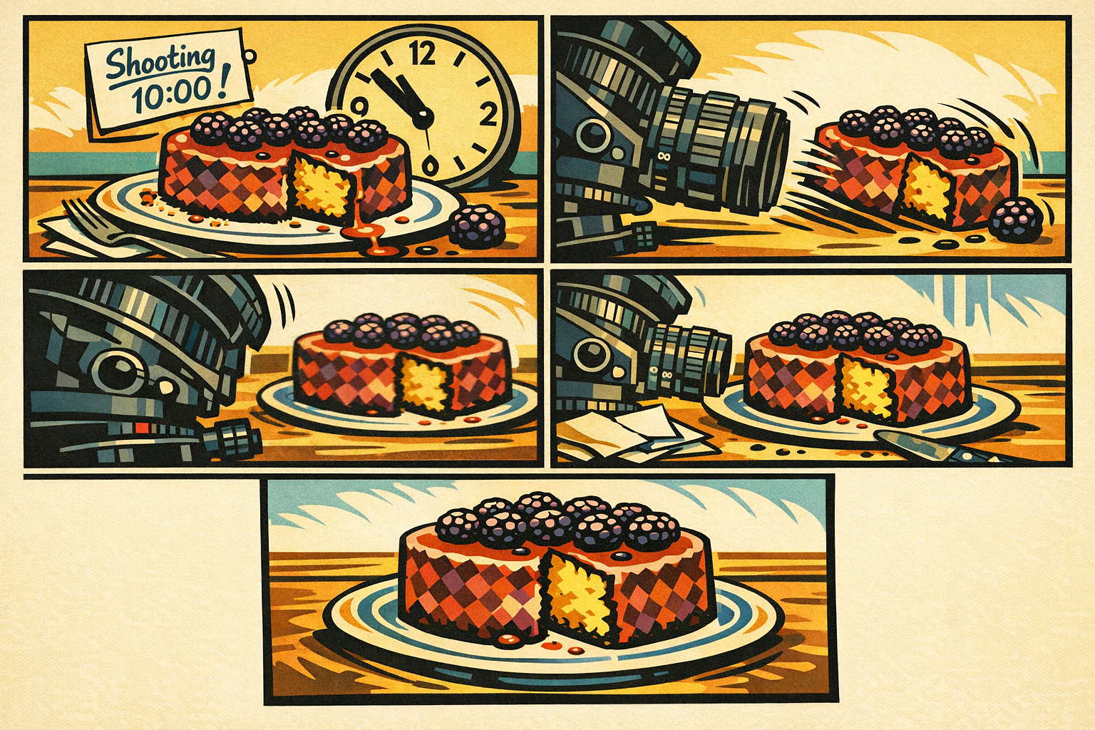
The cake was late for the shoot. One piece was already gone, but there was still time for a quick addition to the family photo album.
In earlier cake sessions, the usual approach was focus stacking: several frames with different focus points, later combined into one final image. That works well, but it also takes time, and this cake was clearly not in the mood for a longer production.
So this time the job went to a tilt adapter and a 35mm2 lens. Instead of building the result from several images, the goal was to get the whole subject sharp in a single frame.
A tilt setup does not simply give more depth of field. What it changes is the angle of the focus plane. Instead of running straight through the scene, the sharp area can be tilted to follow the subject. For something photographed from the side, that makes a real difference. The sharpness no longer has to run mainly from front to back; it can follow the shape of the cake much more naturally.
That is what makes this so interesting. This cannot really be done in software without looking fake. The actual tilt effect has to come from the optics.
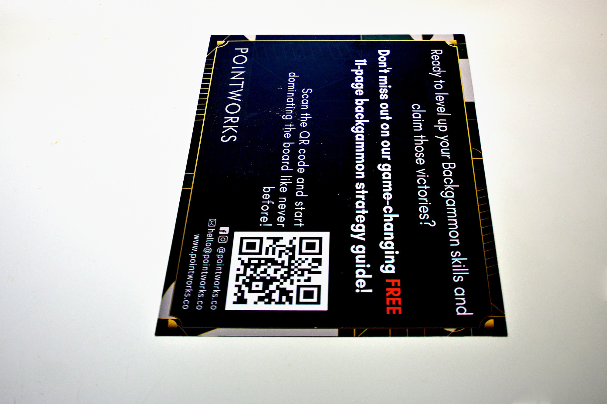
A quick text test
A simple text card as a test subject. With the tilted setup, the whole card stays sharp even though it sits at an angle. The current shooting angle is already very close to the limit of the setup, and at f/2 it gives a good impression of what the tilt adapter can do.
1/40s f/2 ISO 320/26° f=35mm
The Cake
Here is the actual subject. One piece of the round cake is already missing, because cakes do not always wait patiently for the photographic process to begin.
Even the sugar coating tells part of the story, with a few visible traces of a rather hurried arrival.
1/40s f/2 ISO 800/30° f=35mm
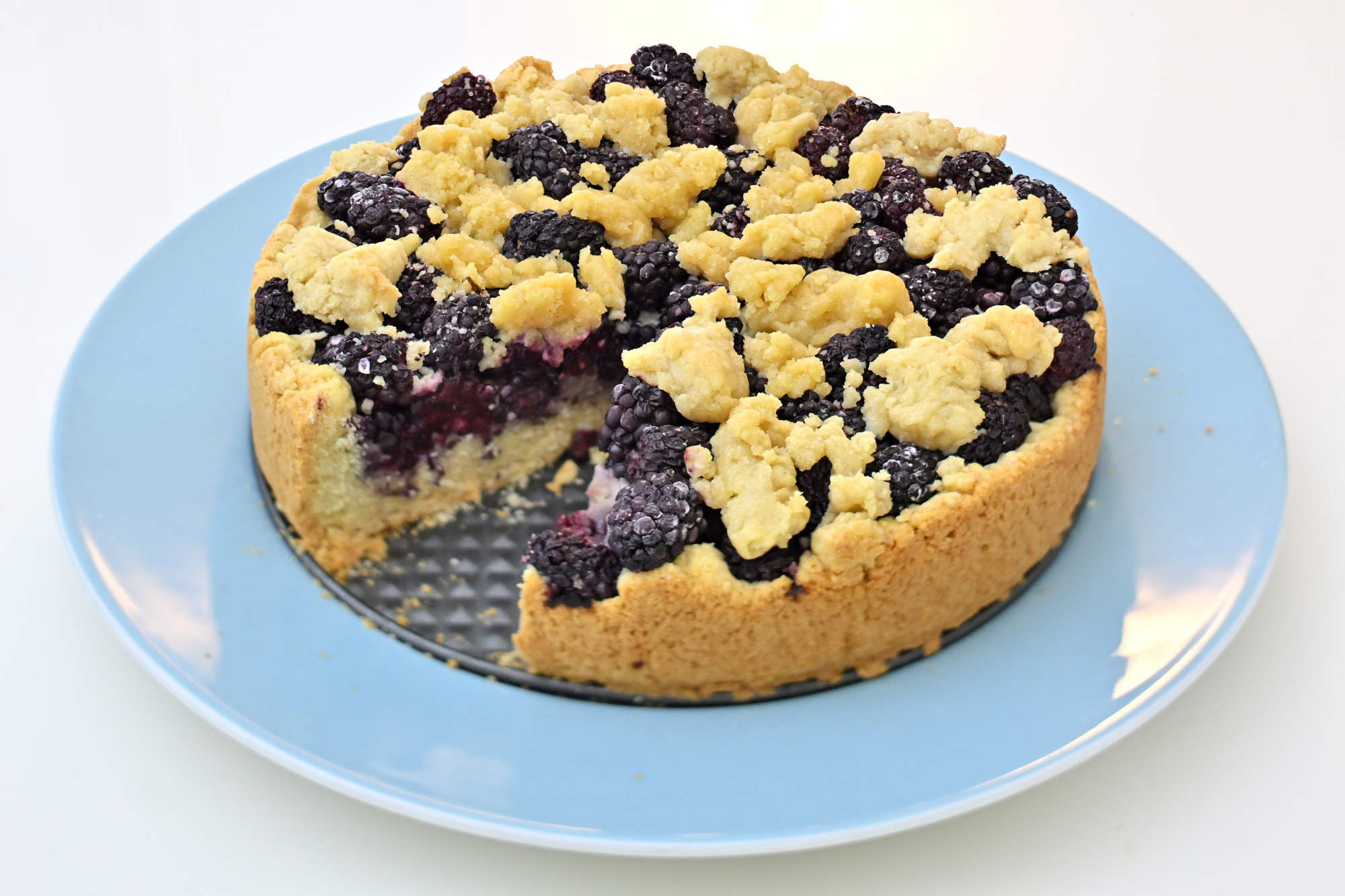
Same angle, no tilt: focus at the front The same view, but with the tilt set to zero. Focus is placed on the front part of the cake, and the rest falls away much more quickly.
1/40s f/2 ISO 320/26° f=35mm
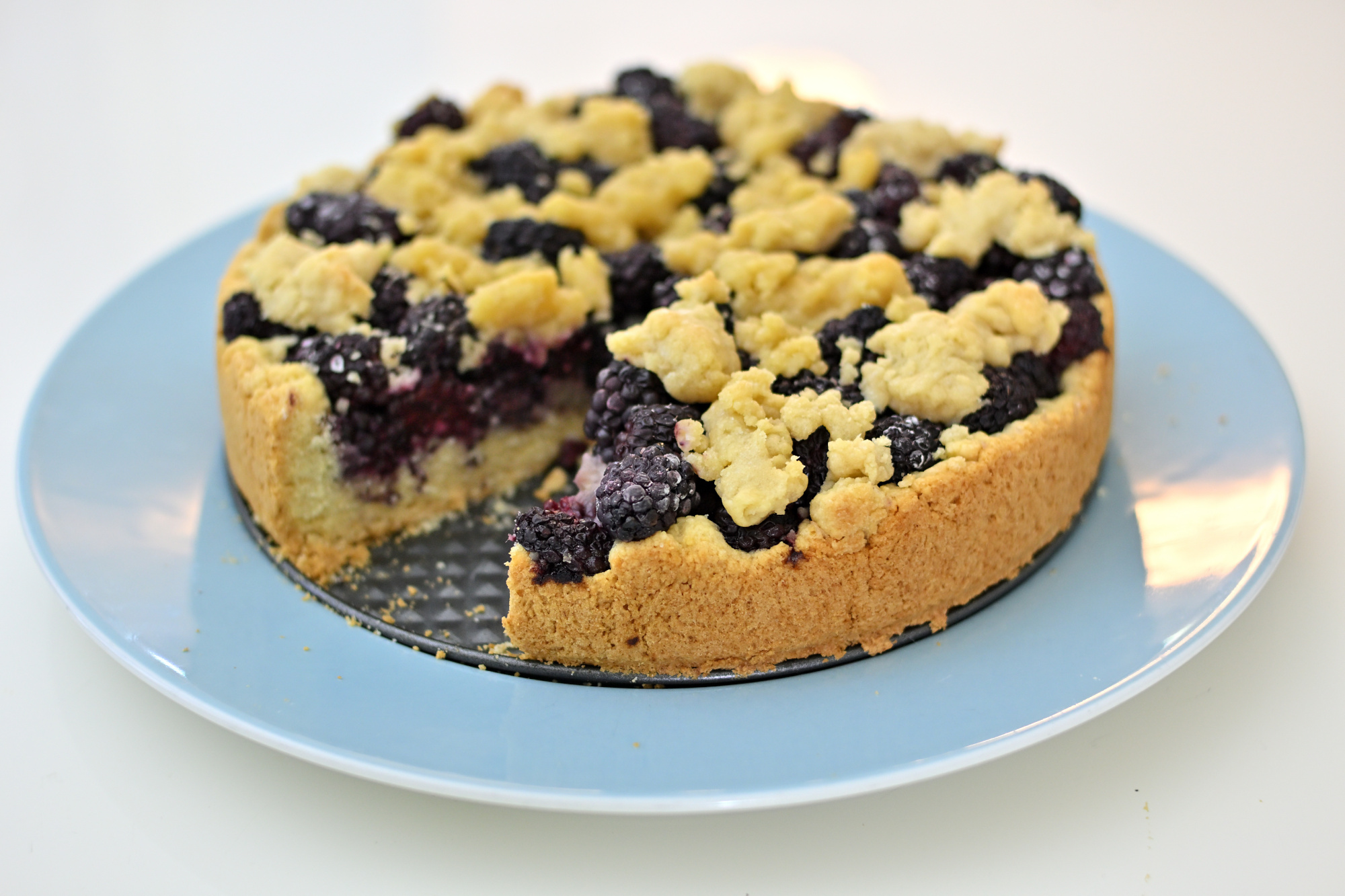
Same angle, no tilt: focus at the back Again the same angle and no tilt, but this time focused farther back. The difference is easy to see, and it shows quite nicely what the tilt setup changes.
1/40s f/2 ISO 320/26° f=35mm
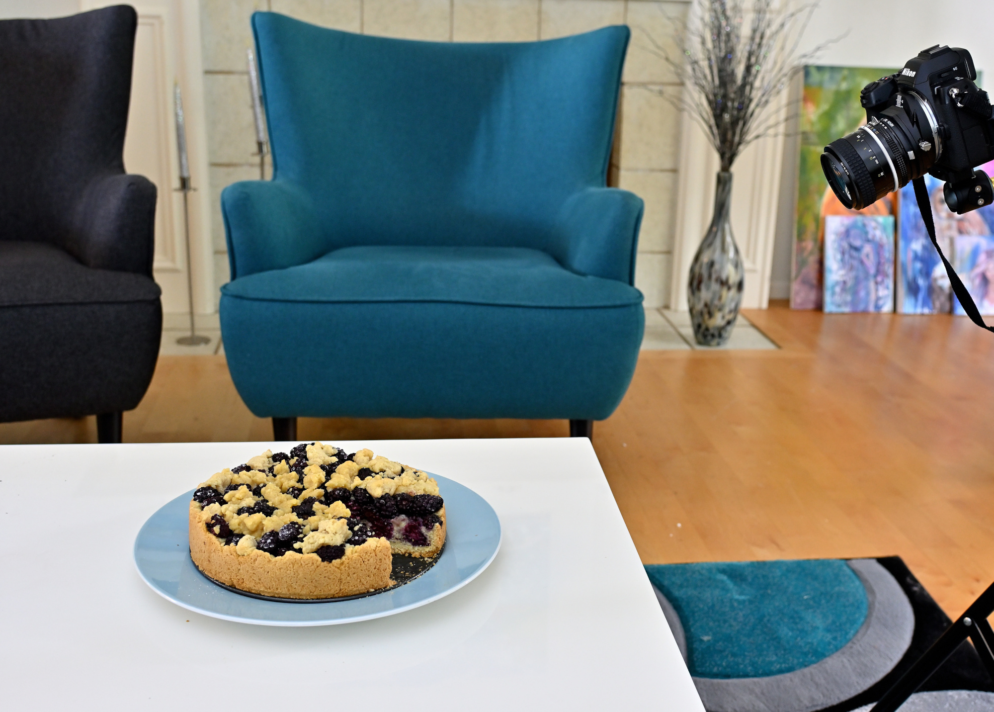
The Setup
The full setup with the cake on the table and the camera floating in the air, carefully aligned and locked onto the target.
1/25s f/4 ISO 400/27° 16-50mm f/2,8 VR f=25mm/37mm
Tilt adapter and 35mm lens
A closer look at the camera with the tilt adapter and the 35mm f/2 lens. A small addition, but one that changes the way this kind of image can be made.
1/30s f/3,2 ISO 400/27° 16-50mm f/2,8 VR f=33mm/50mm
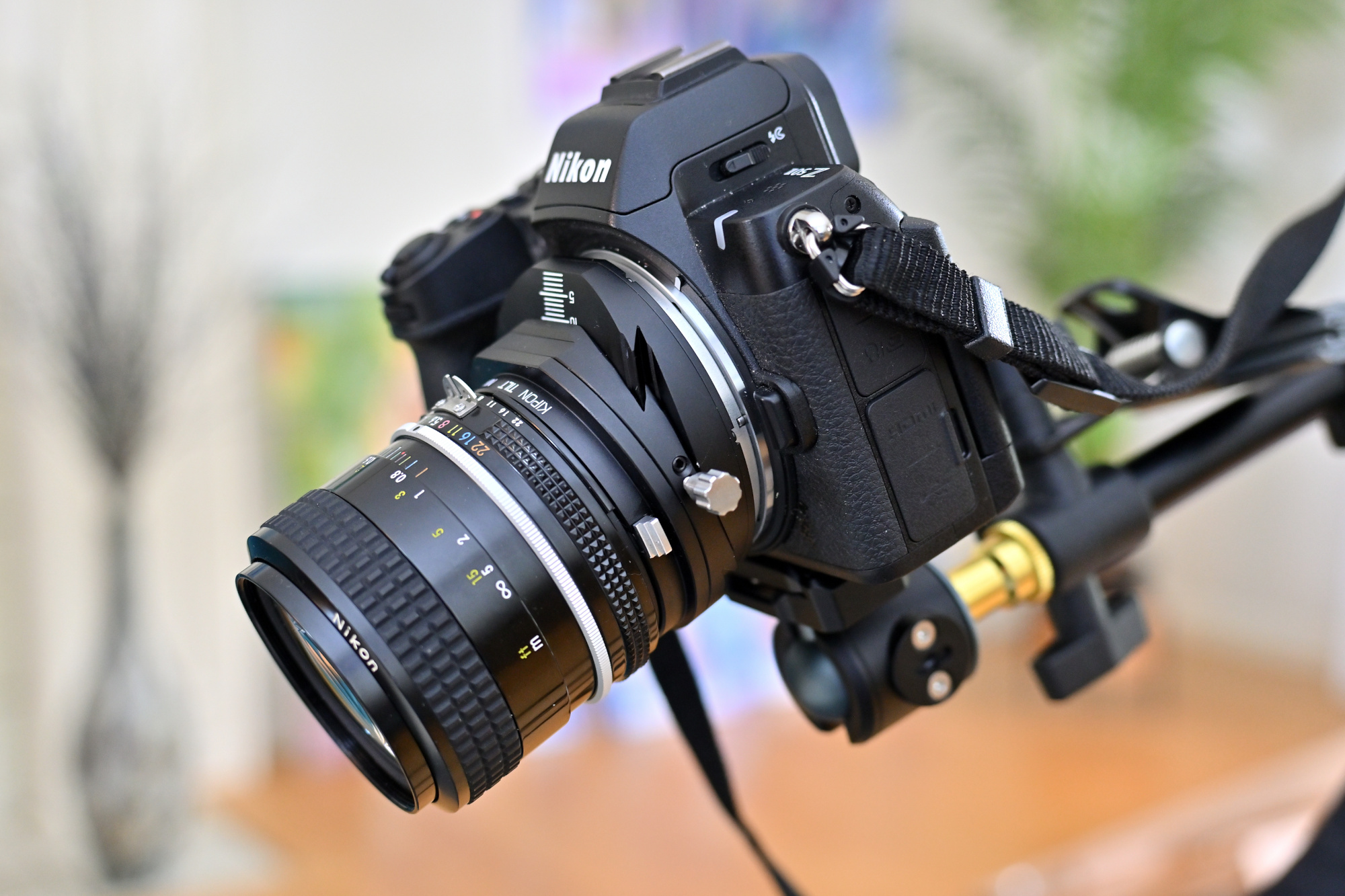
If you look closely, you can still see the fine sand from the Sarasota beaches on the camera. This sand is everywhere. The camera bag did not escape either.
Back on the Coffee Table
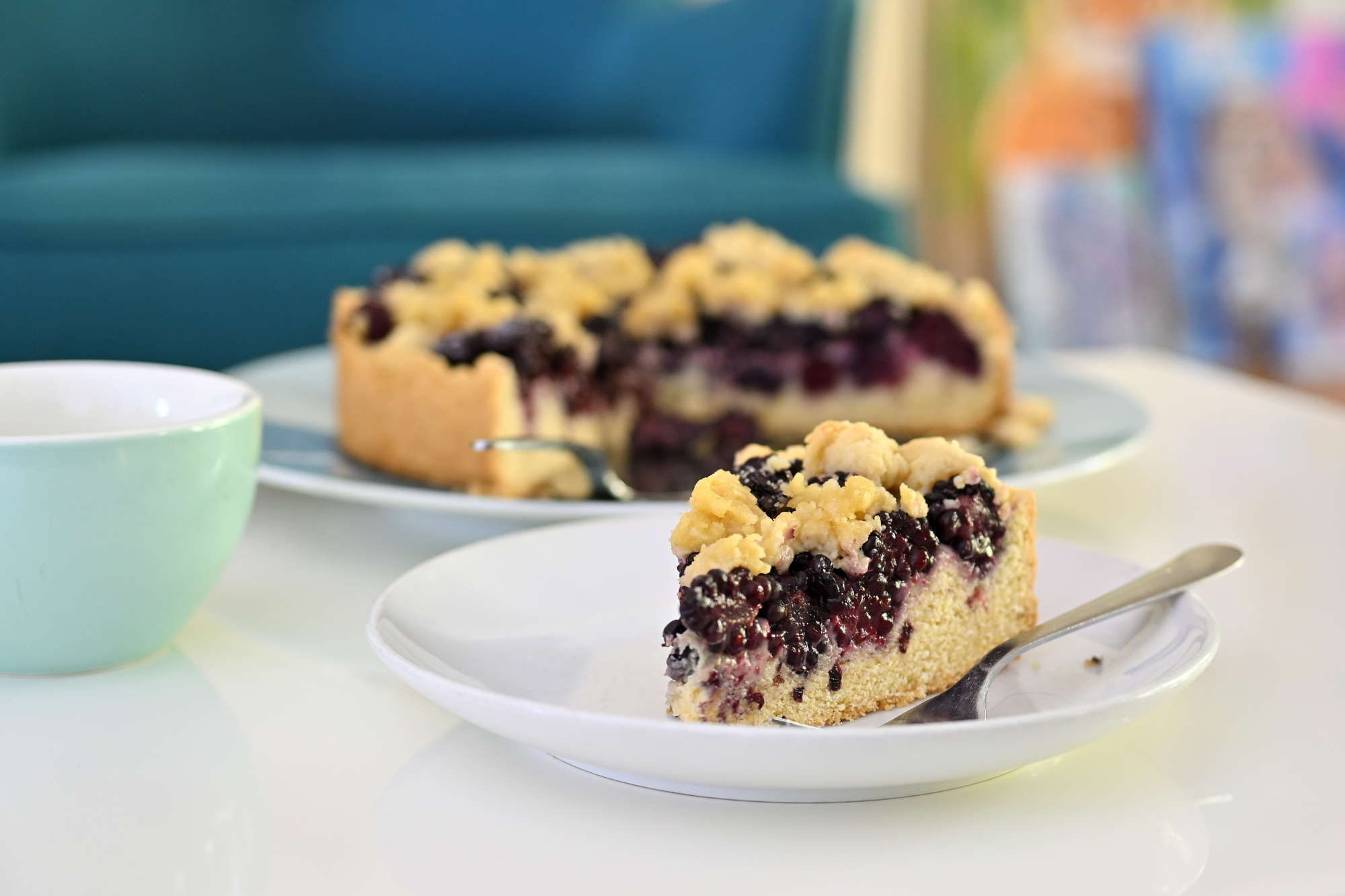
Once the optics had done their job, the cake could finally continue with the coffee part of the story.
1/30s f/2,8 ISO 320/26° 16-50mm f/2,8 VR f=40mm/60mm
-
A Cat at Dusk, ISO 12800
Not every improvement in technology needs a big explanation. Sometimes it is just there in a simple picture taken late in the day, when the light is already fading and everything feels a little softer.
These two photos of our cat were taken at dusk with the Nikon Z50 at ISO 12800 and f/2.8. What I like about them is how calm and natural they feel. The images are sharp, the detail is there, and the whole scene keeps its quiet evening mood.
That is one of the nice things about modern cameras. They make this kind of picture easier and leave more room to focus on the subject, the light, and the moment.
Two quiet moments in the fading evening light
1/80s f/2,8 ISO 12800/42° 16-50mm f/2,8 VR f=50mm/75mm

1/80s f/2,8 ISO 12800/42° 16-50mm f/2,8 VR f=50mm/75mm
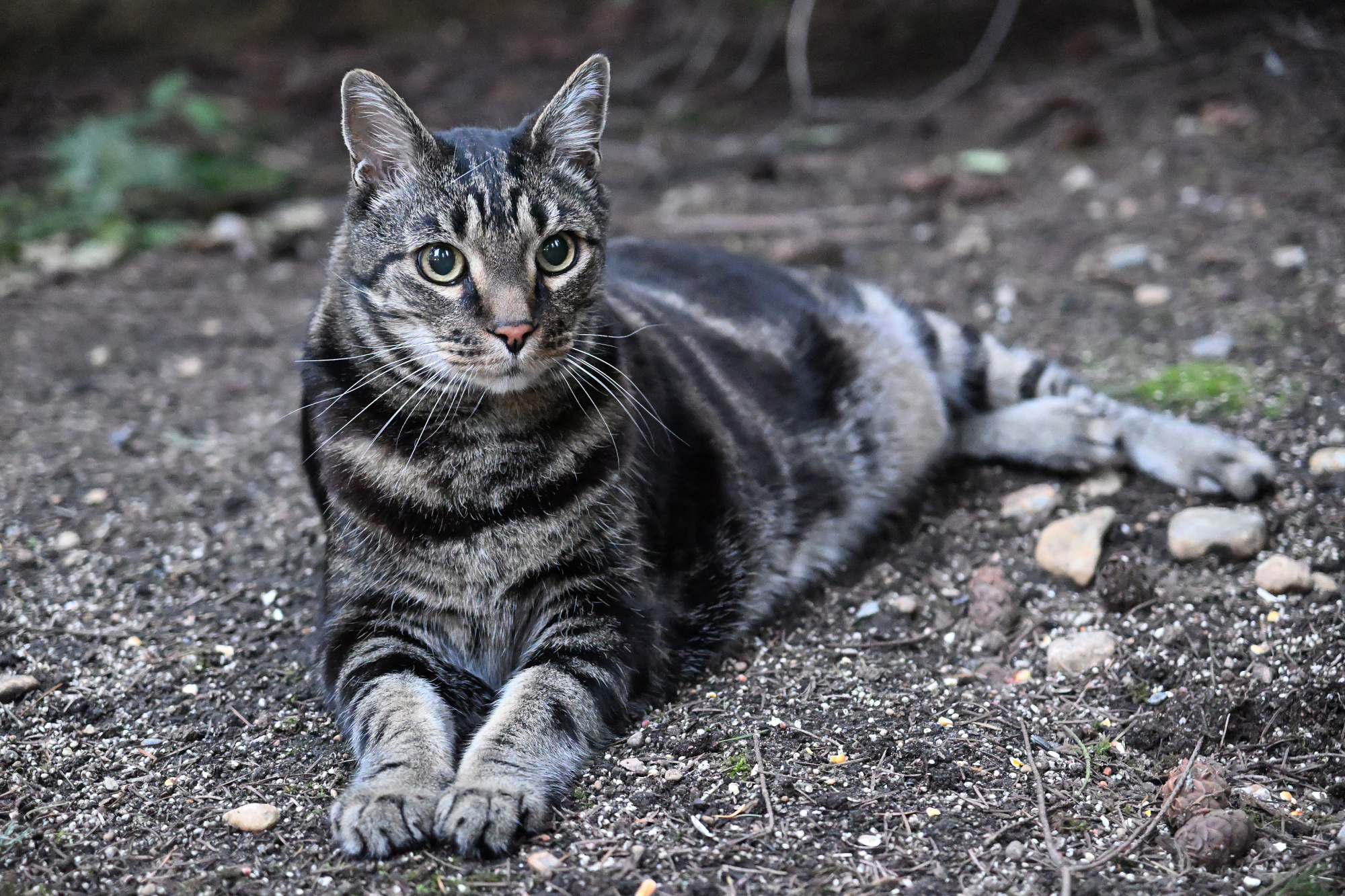
A closer look at the detail, and a nice reminder of how well this works these days.

From the Z50 to JPEG for the web via Nikon NX Studio, with everything left at the default settings.
-
Zwischen Code und Wok: Chow Mein
Chow Mein aus dem Wok 🍜
Nicht alles muss aus Code, Tools und Builds bestehen. Manchmal ist es ganz gut, zwischendurch etwas zu machen, das genauso viel Struktur hat, aber deutlich besser riecht. Diesmal: Chow Mein, also gebratene asiatische Nudeln mit viel Gemüse, Hitze aus dem Wok und genau diesem kurzen Moment, in dem aus einzelnen Zutaten plötzlich ein richtiges Gericht wird.
Ich mag an solchen Gerichten, dass sie schnell wirken, aber trotzdem präzise sind. Alles wird vorbereitet, liegt bereit, und dann geht es Schlag auf Schlag. Fast ein bisschen wie bei einem Deployment: Wenn das Setup stimmt, läuft der Rest sauber durch. Nur eben mit Knoblauch, Sojasauce und Sesamöl statt Logs und Pipelines.
Am Ende ist Chow Mein genau das, was gute Küche oft ist: unkompliziert, direkt und voller Aroma. Hier ein paar Bilder vom Entstehen.
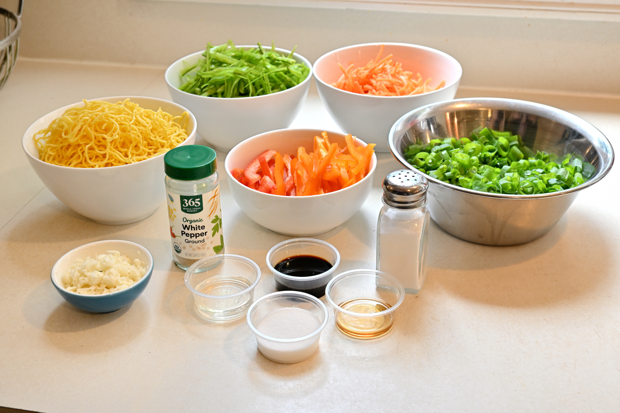
Alle Zutaten im Überblick
Bevor der Wok heiß wird, kommt erst einmal Ordnung auf die Arbeitsfläche: Nudeln, Gemüse, Sauce und alles, was später in wenigen Minuten zusammenfinden soll. Bei so einem Gericht ist die Vorbereitung fast die halbe Miete.
1/40s f/5,6 ISO 100/21° 16-50mm f/2,8 VR f=32mm/48mm
Im Wok: die ersten Schritte
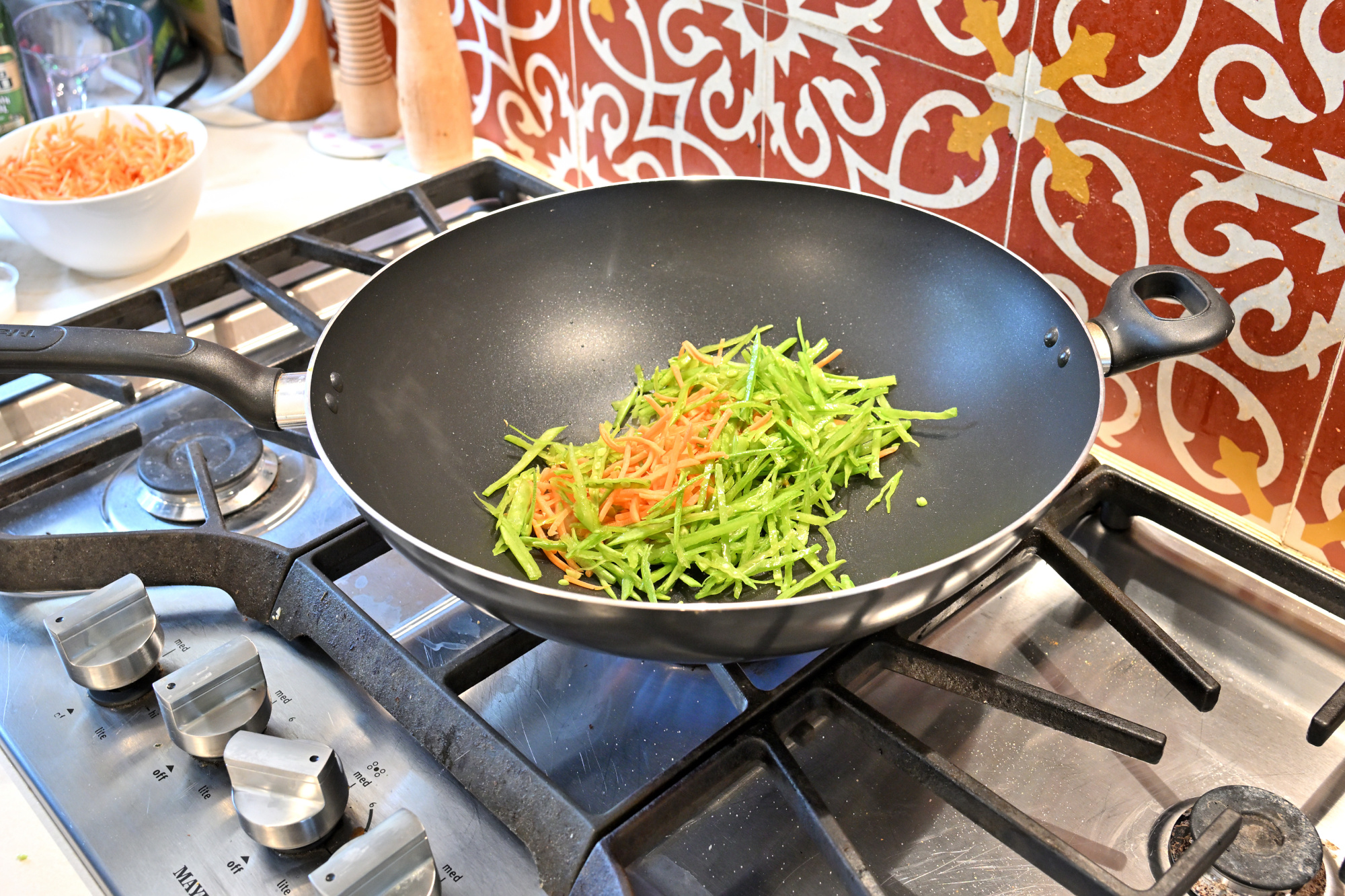
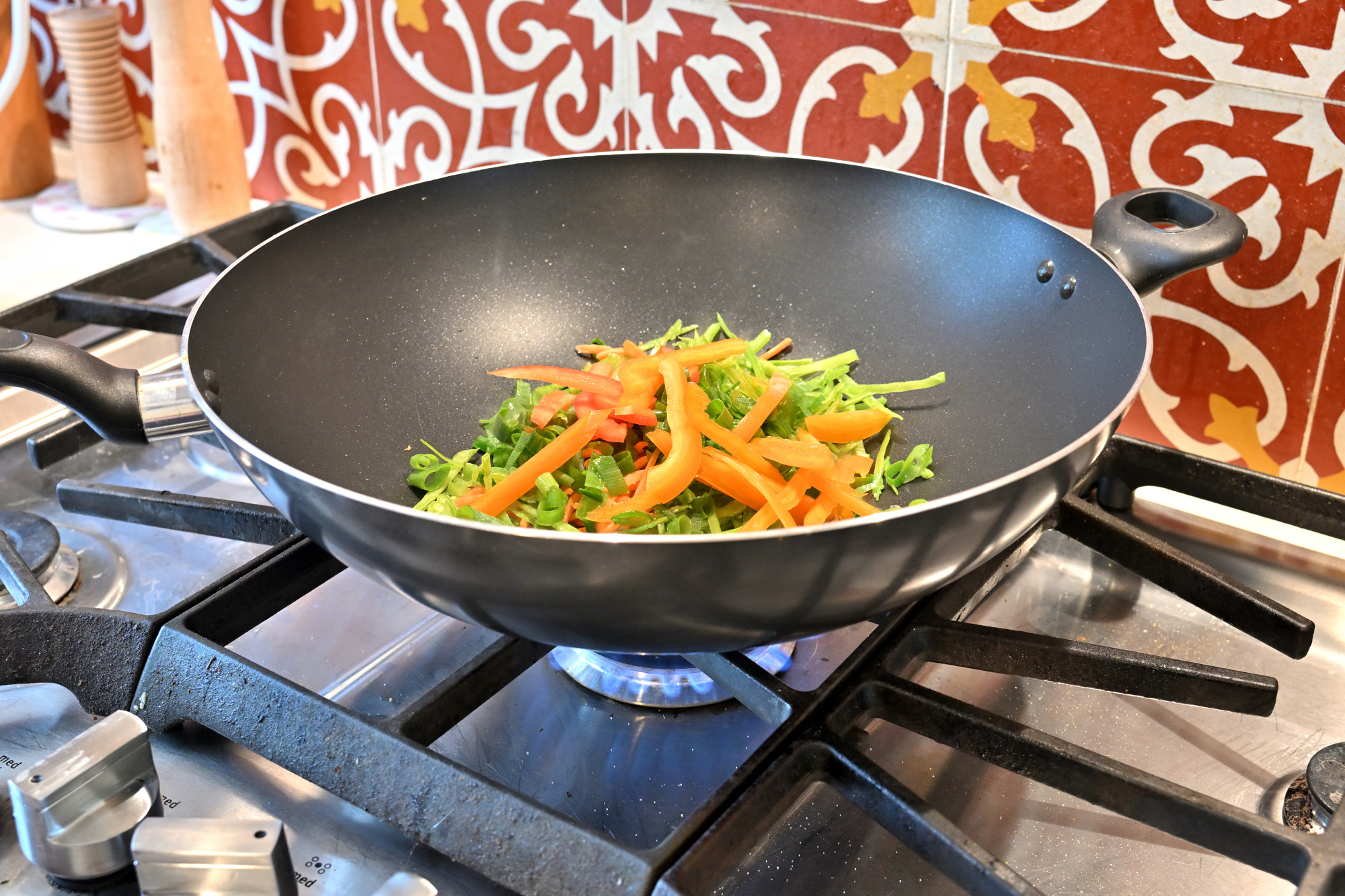
Jetzt wird es ernst. Das Gemüse kommt in den heißen Wok, alles bleibt in Bewegung, und nach den ersten Sekunden entsteht schon dieser typische Duft, bei dem klar ist: Das wird gut.
1/40s f/5 ISO 800/30° 16-50mm f/2,8 VR f=24mm/36mm
1/40s f/5 ISO 800/30° 16-50mm f/2,8 VR f=28mm/42mm
Im Wok: Nudeln und Sauce dazu
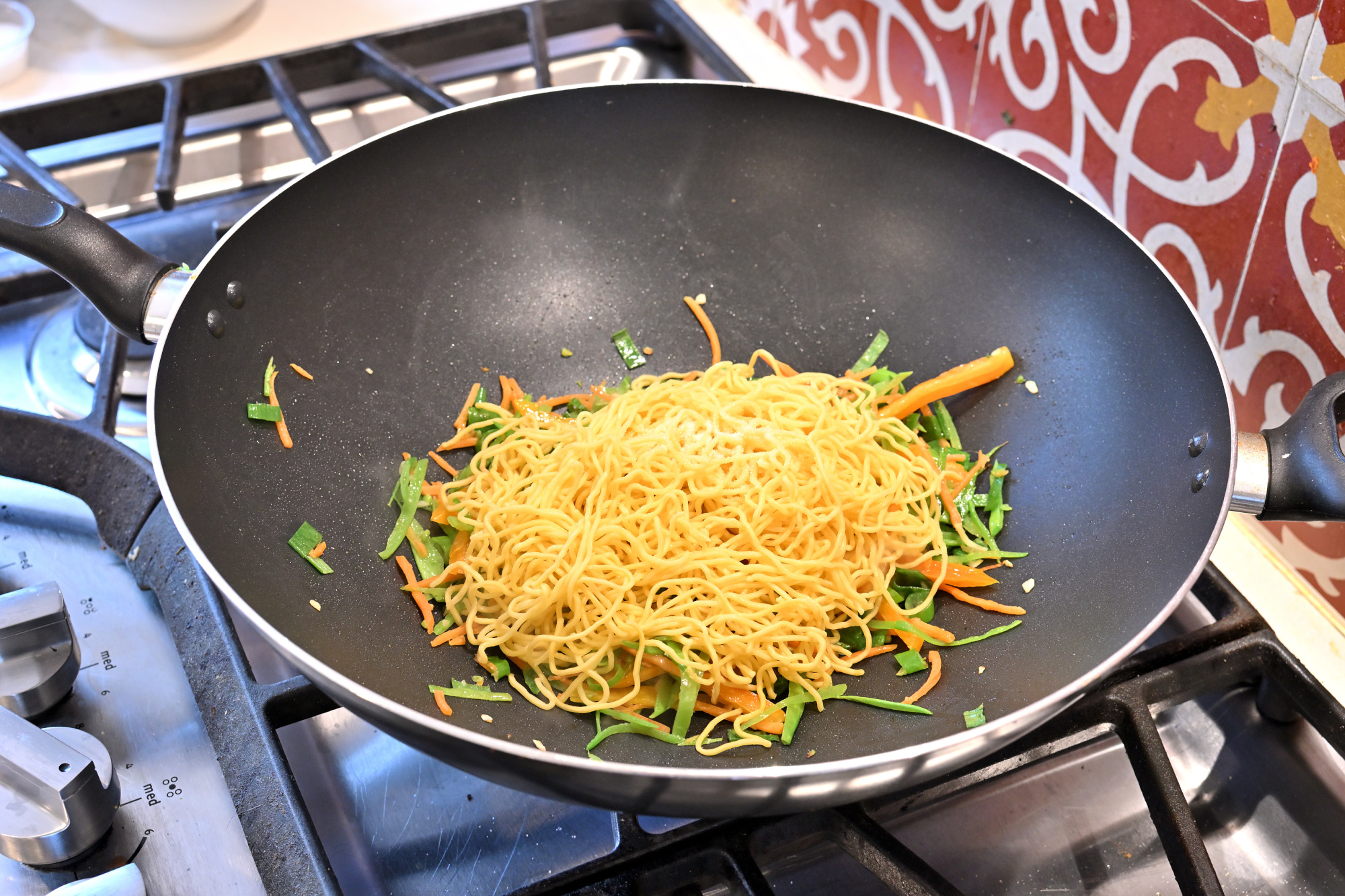
Sobald die Nudeln dazukommen, wird aus Vorbereitung ein Gericht. Die Sauce verbindet alles, der Wok gibt Röstaromen dazu, und plötzlich sieht es nicht mehr nach Zutaten aus, sondern nach Abendessen.
1/40s f/5 ISO 500/28° 16-50mm f/2,8 VR f=32mm/48mm
Kurz vor dem Finale
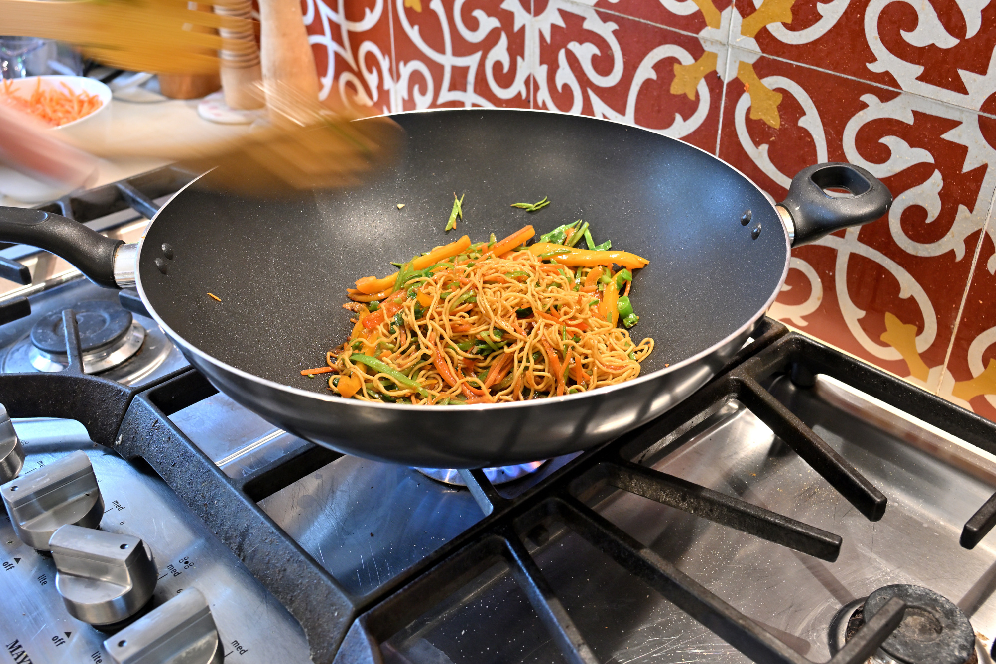
Jetzt passt alles zusammen: Farbe, Struktur und genau die Mischung aus gebraten, saftig und leicht karamellisiert, die Chow Mein ausmacht. Noch ein letzter Schwung im Wok, dann kann angerichtet werden.
1/40s f/5 ISO 500/28° 16-50mm f/2,8 VR f=24mm/36mm
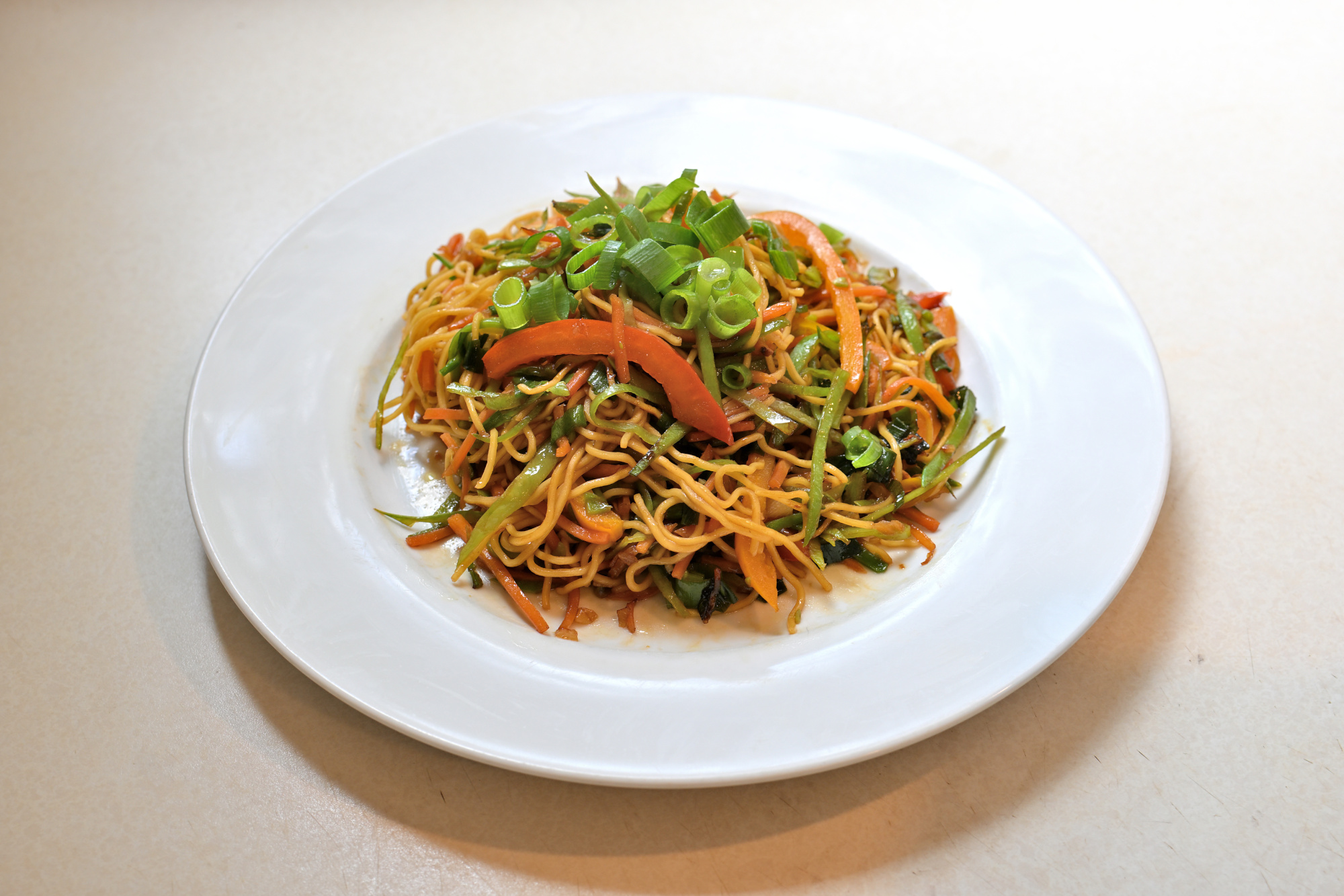
Auf dem Teller
Fertig. Ein Teller Chow Mein, frisch aus dem Wok, heiß, würzig und genau richtig für einen Beitrag, der ausnahmsweise nicht von Technik handelt. Wobei: Ein gutes Ergebnis nach sauberer Vorbereitung ist am Ende doch wieder ziemlich vertraut.
1/40s f/5 ISO 100/21° 16-50mm f/2,8 VR f=33mm/49mm
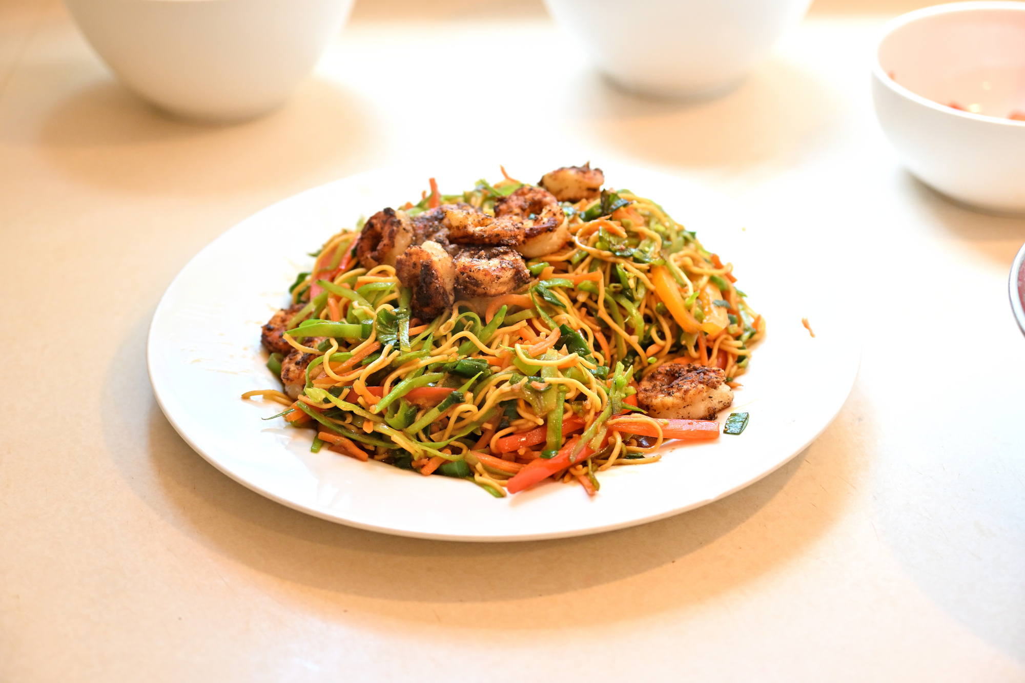
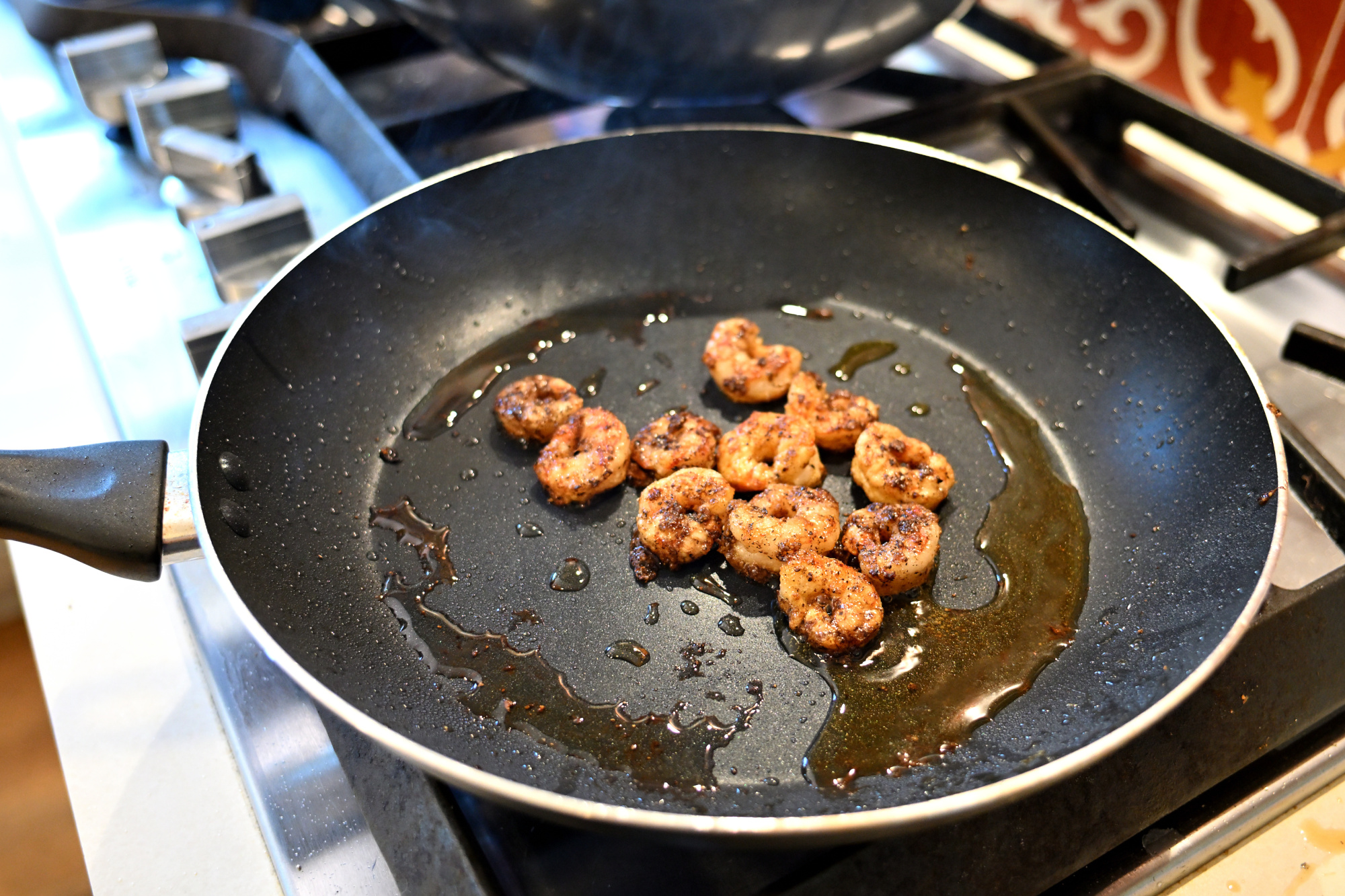
Mit Garnelen
Eine Variante, die dem Gericht nochmal eine etwas andere Richtung gibt. Die Garnelen passen sehr gut zu den gebratenen Nudeln und bringen noch einmal ihren eigenen Charakter mit.
1/125s f/2,8 ISO 1250/32° 16-50mm f/2,8 VR f=22mm/33mm
Fertig angerichtet
Am Teller sieht man dann, wie gut alles zusammenkommt: Farbe, Struktur und genau die Mischung aus Wok-Aroma und frischen Zutaten, die so ein Gericht ausmacht.
1/250s f/2,8 ISO 400/27° 16-50mm f/2,8 VR f=41mm/61mm