Borbin the 🐱

Warum 50 Ohm? Die Physik hinter dem HF-Standard

Wer zum ersten Mal ein Koaxialkabel in der Hand hält und auf dem Aufdruck "50 Ω" liest, fragt sich unweigerlich: Warum ausgerechnet 50? Die Antwort liegt in einem eleganten Kompromiss zwischen zwei physikalischen Optima und etwas Militärgeschichte.

Das Ergebnis vorweg

Für ein Koaxialkabel mit Luft als Dielektrikum gibt es zwei physikalisch optimale Wellenwiderstände, je nach Ziel:

Das geometrische Mittel liegt bei:

$$Z_0 = \sqrt{77\,\Omega \times 30\,\Omega} \approx 48\,\Omega$$

Das geometrische Mittel ist hier sinnvoller als das arithmetische, weil Impedanzen auf einer logarithmischen Skala natürlich sind. Das geometrische Mittel minimiert den maximalen relativen Abstand zu beiden Optima gleichzeitig. Das Ergebnis wurde auf 50 Ω gerundet und Anfang der 1930er Jahre als militärischer Standard etabliert (MIL-SPEC, später von IEC und IEEE übernommen).

Grundlagen: Wellenwiderstand einer Leitung

Die Telegrafengleichungen

Eine reale Leitung lässt sich nicht als einfacher Draht beschreiben, denn Spannung und Strom ändern sich entlang der Leitung. Das Modell: jedes infinitesimale Stück $dx$ verhält sich wie ein kleines LC-Glied:

───L'dx───┬───
          C'dx
          │
──────────┴───

$L'$ = Induktivitätsbelag, $C'$ = Kapazitätsbelag (jeweils pro Längeneinheit). Aus den Kirchhoffschen Regeln auf diesem verteilten Netzwerk folgen die Telegrafengleichungen:

$$-\frac{\partial u}{\partial x} = L' \frac{\partial i}{\partial t}, \qquad -\frac{\partial i}{\partial x} = C' \frac{\partial u}{\partial t}$$

Von den Telegrafengleichungen zur Wellengleichung

Differenziert man die erste Gleichung nach $x$ und setzt die zweite ein:

$$\frac{\partial^2 u}{\partial x^2} = L' \frac{\partial}{\partial t}\left(-\frac{\partial i}{\partial x}\right) = L' C' \frac{\partial^2 u}{\partial t^2}$$

Das ist die Wellengleichung mit Phasengeschwindigkeit $v = 1/\sqrt{L'C'}$.

Wellenwiderstand $Z_0 = \sqrt{L'/C'}$

Für eine harmonische Welle $\sim e^{j(\omega t - kx)}$ gilt $\partial/\partial x \to -jk$ und $\partial/\partial t \to j\omega$. Einsetzen in die erste Telegrafengleichung:

$$jk \cdot U = j\omega L' \cdot I \quad \Rightarrow \quad Z_0 = \frac{U}{I} = \frac{\omega L'}{k}$$

Mit der Dispersionsrelation $k = \omega/v = \omega\sqrt{L'C'}$:

$$\boxed{Z_0 = \frac{\omega L'}{\omega\sqrt{L'C'}} = \sqrt{\frac{L'}{C'}}}$$

$Z_0$ ist also das Verhältnis von Spannung zu Strom einer laufenden Welle, eine reine Geometrieeigenschaft, keine Last. Eine reflexionsfreie Terminierung mit $Z_\text{Last} = Z_0$ lässt die Leitung „unendlich lang" erscheinen.

$L'$ und $C'$ für das Koaxialkabel

Innenleiter-Radius $a$, Außenleiter-Radius $b$. Beide Felder sind rotationssymmetrisch und exakt berechenbar:

Induktivitätsbelag (aus dem Ampèreschen Gesetz: Magnetfeld $B(r) = \mu_0 I / 2\pi r$, Integration von $a$ bis $b$):

$$L' = \frac{\mu_0}{2\pi} \ln\!\left(\frac{b}{a}\right)$$

Kapazitätsbelag (aus dem Gaußschen Gesetz: elektrisches Feld $E(r) = \lambda / 2\pi\varepsilon_0 r$, Spannung durch Integration):

$$C' = \frac{2\pi\varepsilon_0}{\ln(b/a)}$$

Einsetzen in $Z_0 = \sqrt{L'/C'}$:

$$Z_0 = \sqrt{\frac{\mu_0}{2\pi}\ln\!\left(\frac{b}{a}\right) \cdot \frac{\ln(b/a)}{2\pi\varepsilon_0}} = \frac{\ln(b/a)}{2\pi}\sqrt{\frac{\mu_0}{\varepsilon_0}}$$

Wellenwiderstand des Vakuums

$$Z_\text{Vak} = \sqrt{\frac{\mu_0}{\varepsilon_0}} \approx 376{,}73\,\Omega$$

Mit $x = b/a$:

$$Z_0 = \frac{376{,}73}{2\pi} \cdot \ln(x) \approx 59{,}95 \cdot \ln(x) \approx \boxed{60 \cdot \ln(x) \quad [\Omega]}$$

Mit Dielektrikum ($\varepsilon_r > 1$) ersetzt $\varepsilon_0 \to \varepsilon_0\varepsilon_r$:

$$Z_0 = \frac{60}{\sqrt{\varepsilon_r}} \cdot \ln(x)$$

Für Luft ($\varepsilon_r \approx 1$) entfällt der Faktor.

Herleitung der optimalen Impedanzen

1. Minimale Dämpfung

Die Dämpfungskonstante $\alpha$ beschreibt, wie stark die Amplitude pro Längeneinheit abnimmt:

$$U(z) = U_0 \cdot e^{-\alpha z}$$

Die Dämpfung entsteht durch den ohmschen Widerstand beider Leiter. Wegen des Skin-Effekts fließt der Strom hierbei nur in einer dünnen Schicht der Tiefe $\delta = \sqrt{2/(\omega\mu\sigma)}$ an der Oberfläche. Der Widerstandsbelag ist damit:

$$R' = \frac{1}{2\pi\sigma\delta}\left(\frac{1}{a}+\frac{1}{b}\right)$$

Mit $\alpha = R'/(2Z_0)$ und nach Kürzen aller Konstanten hängt $\alpha$ nur noch von der Geometrie ab:

$$\alpha \propto \frac{1/a + 1/b}{\ln(b/a)} = \frac{x+1}{\ln(x)}, \quad x = \frac{b}{a}$$

(Außenleiter $b$ fest, $a = b/x$ variabel, Faktor $1/b$ kürzt sich heraus.)

Minimum durch Nullsetzen der Ableitung:

$$\frac{d}{dx}\left[\frac{x+1}{\ln x}\right] = \frac{\ln x - \dfrac{x+1}{x}}{\ln^2 x} = 0 \quad \Rightarrow \quad \ln x = 1 + \frac{1}{x}$$

Numerisch: $x \approx 3{,}6$ → $Z_0 = 60 \cdot \ln(3{,}6) \approx \mathbf{77\,\Omega}$

2. Maximale Leistung

Die maximale übertragbare Leistung wird durch die Durchschlagsfeldstärke am Innenleiter begrenzt. Das elektrische Feld im Koaxialkabel folgt aus dem Gaußschen Gesetz (Zylindersymmetrie):

$$E(r) = \frac{V}{r \cdot \ln(b/a)}$$

Da $E(r) \propto 1/r$, ist das Feld am Innenleiter ($r = a$) am stärksten, dort tritt zuerst Durchschlag auf:

$$E_\text{max} = \frac{V}{a \cdot \ln(b/a)} \quad \Rightarrow \quad V = E_\text{max} \cdot a \cdot \ln x$$

Die übertragbare Leistung bei gegebenem $E_\text{max}$:

$$P = \frac{V^2}{2Z_0} \propto \frac{(a \cdot \ln x)^2}{\ln x} = a^2 \cdot \ln x$$

Mit $a = b/x$ (Außenleiter $b$ fest):

$$P \propto \frac{\ln x}{x^2}$$

Maximum durch Nullsetzen der Ableitung:

$$\frac{d}{dx}\left[\frac{\ln x}{x^2}\right] = \frac{1 - 2\ln x}{x^3} = 0 \quad \Rightarrow \quad \ln x = \frac{1}{2} \quad \Rightarrow \quad x = \sqrt{e} \approx 1{,}65$$

$$Z_0 = 60 \cdot \ln(\sqrt{e}) = 60 \cdot \frac{1}{2} = \mathbf{30\,\Omega}$$

Zusammenfassung der Optima

Warum dennoch nicht 30 Ω für Hochleistungssender?

1. Standardisierung dominiert
Die gesamte HF-Infrastruktur (Koaxkabel, Stecker, Messgeräte, Verstärker) ist auf 50 Ω ausgelegt. Ein Sender mit 30 Ω bräuchte überall Transformatoren → Verluste und Kosten.

2. Das Leistungsoptimum ist sehr flach
Die Kurve, die die maximale Leistungsübertragung beschreibt, fällt in Richtung 50 Ohm nur sehr flach ab. Der Verlust an maximaler Sendeleistung ist im Alltag also minimal (nur wenige Prozent schlechter als bei 30 Ω), weshalb es keinen wirtschaftlichen Vorteil bringt.

3. Mechanische Grenzen
$D/d \approx 1{,}65$ bedeutet: der Innenleiter ist fast so dick wie der Außenleiter. Das ergibt wenig Isolationsabstand und ist schwer zu fertigen.

4. Hochleistungssender verwenden Hohlleiter
Bei echten Hochleistungsanlagen (MW, kW-Bereich) verwendet man Hohlleiter statt Koaxkabel. Dort gelten völlig andere Optimierungskriterien.

Stattdessen haben sich je nach Anwendung zwei Standards etabliert:

75 Ω ist höherohmig als 50 Ω und näher am Dämpfungsoptimum und sinnvoll dort, wo nur kleine Empfangssignale übertragen werden und jeder Verlust zählt.

Connecting AI to the Physical World with Model Context Protocol

As detailed in StickyMCP: Notes That Stick, Even in the Cloud, MCP servers open the door for AI systems to interact with real-world tools far beyond their usual diet of static training data and existential boredom.

This project brings together two cutting-edge technologies: the Model Context Protocol (MCP) and Arduino Microcontroller. The result is an MCP server running directly on an Arduino Nano ESP32, allowing AI assistants control physical hardware in real-time.

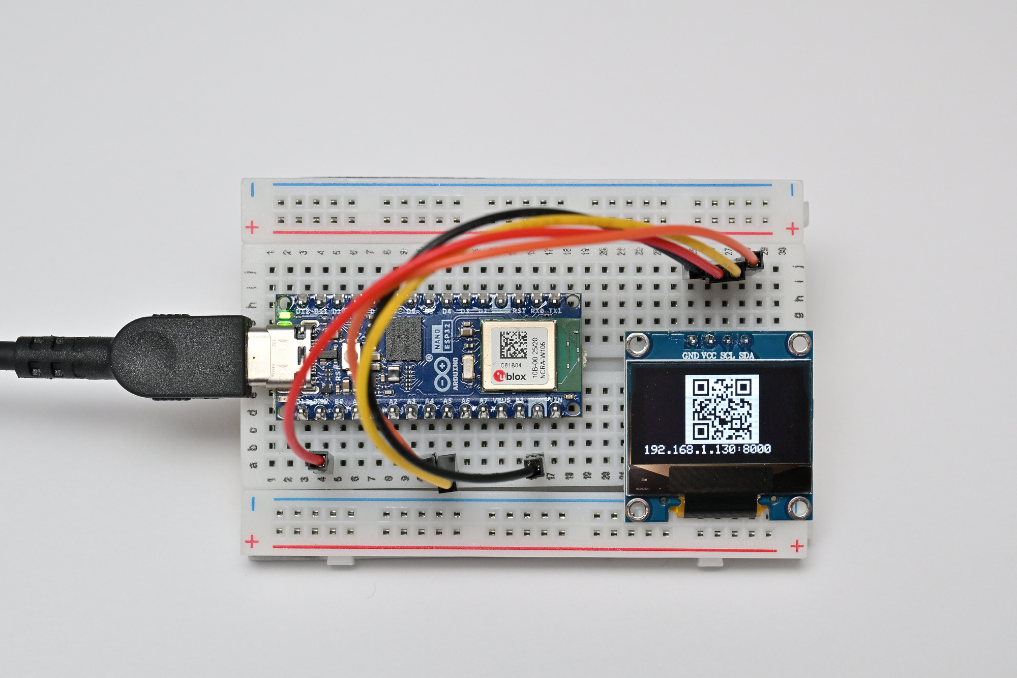
(Some prompts were typed a bit wrong because I had the camera in the way, but Copilot Chat did not mind at all)

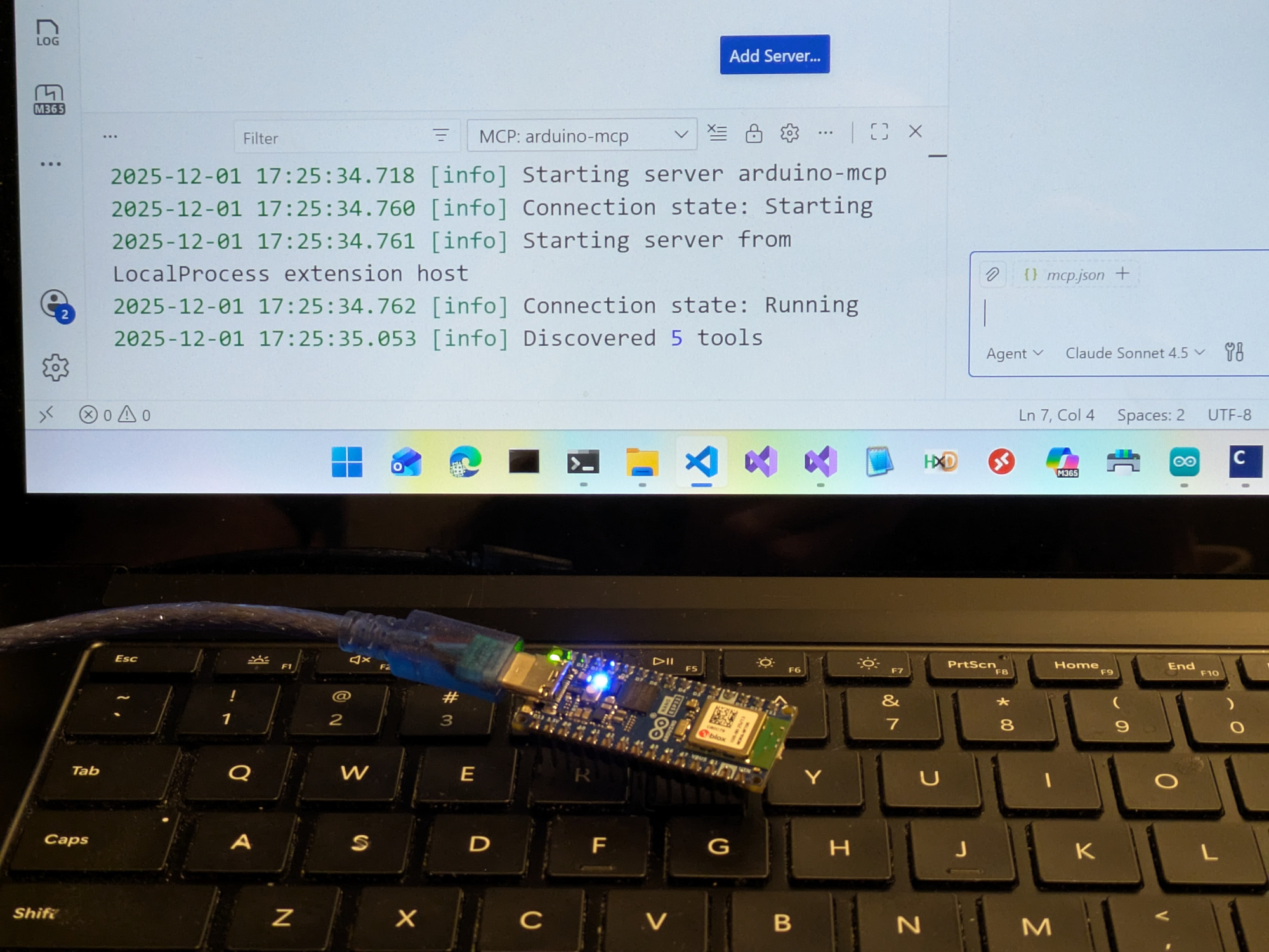
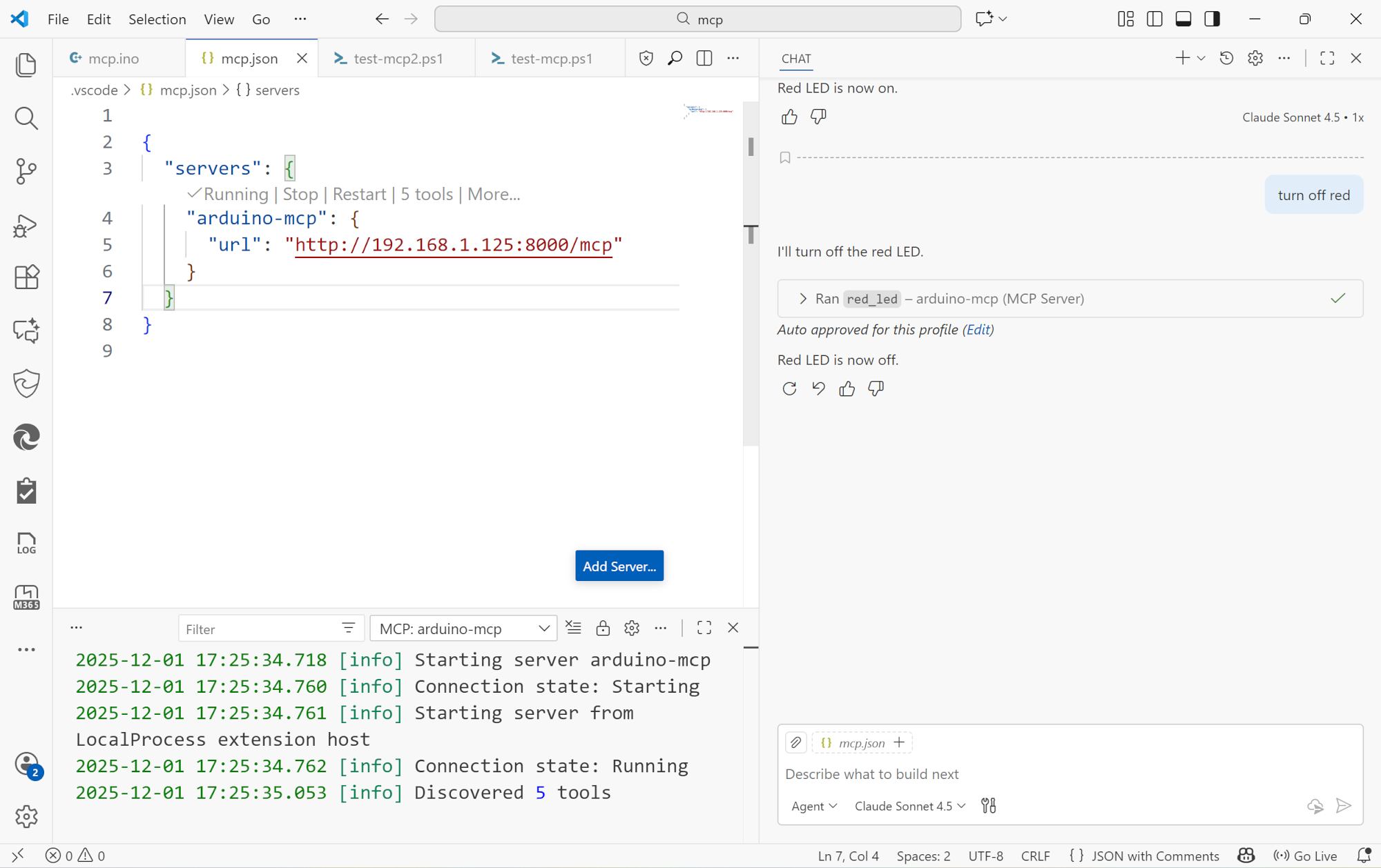
Since no official C++ MCP SDK exists, I built one optimized for embedded systems. Features automatic JSON schema generation, registry-based tool discovery, and memory-safe execution. Architecture mirrors official SDKs (TypeScript/Python) while addressing embedded constraints. Demonstrates full MCP protocol compliance with hardware control tools. I kept it small and readable, and made it work to run simple tools like switching lights on and off.

esp32-mcp on github

What is it?

This project implements a fully-compliant JSON-RPC 2.0 MCP server on an Arduino Nano ESP32 microcontroller. It exposes hardware controls (LEDs in this case) as MCP "tools" that can be invoked by AI assistants through natural language commands.

Key Features

• MCP Protocol Support: Implements the MCP 2024-11-05 specification with proper initialization, tool listing, and tool execution
• JSON-RPC 2.0 Compliance: Standard protocol interface for reliable communication
• WiFi-Enabled: Runs a web server on port 8000, making it accessible over the network
• Server-Sent Events (SSE): Real-time notifications and logging stream for monitoring
• Multiple LED Controls: Manages built-in LED plus RGB LEDs (red, green, blue) independently
• Echo Tool: Simple text echo for testing and demonstration

Technical Implementation

The server uses the ESPAsyncWebServer library for handling HTTP requests and ArduinoJson for JSON parsing/serialization. It exposes two main endpoints:

• POST /mcp - Main JSON-RPC 2.0 endpoint for all MCP methods
• GET /sse - Server-Sent Events stream for real-time notifications

Each LED is implemented as an MCP tool with a simple boolean parameter to turn it on or off. The server handles all the MCP lifecycle methods including initialization, capability negotiation, and tool invocation.

Real-World Applications

This project demonstrates how AI assistants can seamlessly control physical devices. Instead of writing custom scripts or manual API calls, you can simply tell an AI assistant "turn on the red LED" and it happens. This opens up possibilities for:

• Smart home automation controlled by natural language
• Laboratory equipment control through AI assistants
• Educational demonstrations of AI-hardware integration
• Rapid prototyping of IoT devices with conversational interfaces

Technical Stack:

• Arduino Nano ESP32
• ESPAsyncWebServer
• ArduinoJson
• Model Context Protocol (MCP) 2024-11-05
• JSON-RPC 2.0

Precise timing is critical in analog photography, especially during the development process in the darkroom. This project presents a versatile darkroom timer built around the Arduino Uno R4 and Gamepad Input Shield, designed to support key photographic development tasks with tactile control and visual feedback. It features an 8x8 LED matrix for ambient illumination and implements five distinct modes: LED brightness adjustment, manual and timed enlarger control, chemical bath sequencing, and a general-purpose timer. Navigation is intuitive via joystick or button input, making it a practical and user-friendly tool for analog photography workflows.

This project uses the Gamepad Input Shield and Arduino Uno R4. Wiring details are available in the source code. The joystick or up/down buttons are used to switch between tasks, while left/right buttons adjust the state or settings.
The first 8x8 LED block is used to illuminate the darkroom.

The timer implements five tasks:

• LEDBrightnessTask: Adjusts LED brightness from 0 to 15.
• EnlargerOnOffTask: Manual control of the enlarger.
• EnlargerTimerTask: Timed control of the enlarger.
• DevelopStopFixTask: Three timers for develop, stop bath, and fix stages.
• GeneralTimerTask: A general-purpose timer starting from 0 seconds.

LEDBrightnessTask

Sets the brightness of the 8x8 darkroom illumination LEDs from min 0 to max 15.

EnlargerOnOffTask

Manual enlarger switch switched on.

EnlargerTimerTask

Timed enlarger switch.

DevelopStopFixTask

3 timers for develop, stop bath and fix.

GeneralTimerTask

General timer starting from 0s.

Arduino Darkroom Timer Github Project

This darkroom timer project combines modern microcontroller technology with the tactile simplicity of gamepad input to support essential analog photography tasks. Whether you are timing enlarger exposures or chemical baths, this tool offers consistent performance and flexibility for both amateur and professional darkroom enthusiasts. With five dedicated modes and intuitive controls, it provides a reliable and customizable solution for anyone working in a traditional darkroom. The open-source design invites further experimentation and adaptation. Whether you are refining your workflow or building your own version.

The new Arduino MKR 1010 was released this year and supports wireless connection. It is similar to the M0 Pro, in that it also uses a SAMD21 32bit processor. It is much smaller but has the same amount of I/O pins available as the M0 Pro.
I had to try it out!

The previous setup was using an Ethernet shield that connected the controller by cable with the router.

I moved everything to an experimental board and switched out the Ethernet class and replaced it with the new Wifi class, along with a few other changes to get it working.

The bright spot in the middle of the board is actually a RGB LED of the wireless controller! I use each of the three colors to indicate HTTP requests, update of time and wind data and update of the air pressure, humidity and temperature.
Out of a brightness range from 1..255, 7 seems a good value to match the internal yellow LED.
It is also possible to use a digitalWrite on the LED port to switch it on or off. This is the same as using analogWrite with 255. This is very bright.

const int GREEN_LED = 25;
const int RED_LED = 26;
const int BLUE_LED = 27;
const int LED_Brightness = 7;

// Configure the LED port of the wireless controller.
WiFiDrv::pinMode(GREEN_LED, OUTPUT);
WiFiDrv::pinMode(RED_LED, OUTPUT);
WiFiDrv::pinMode(BLUE_LED, OUTPUT);

// Set the LED.
WiFiDrv::analogWrite(GREEN_LED, bGreenLed ? LED_Brightness : 0);

The webserver on the board provides a full HTML page and the weather data in a json format for the AJAX requests that gets updated every second.

The matching App is using the AJAX data for display

and also provides access to the weather data for wind, temperature and air pressure stored in the 32Kb chip.

Using a Arduino M0 Pro to power a weather station to measure wind speed/direction, humidity and temperature inside and outside, barometric pressure and rainfall, support REST API for the weather app and HTTP Server:

The white sensor is a DHT22 to measure the humidity and temperature inside.

The 8 pin DIP on the experimental board is a 24LC256 (32KB) to hold weather data statistics.
The wireless module is already connected and will be used later to upload data to the Azure IOT hub.

First test with the weather station to check the directional sensor and the areometer signal.
The weather station is a very popular model, but the documentation has a wrong value for the resistance for one direction.
Here is the correct list:

This translates to the following analog values using the recommended 10K resistor. The analog2index function returns the index (the wind direction) of the received value from the Arduino analog input port. Since the differences between the individual values is not constant, this mapping is the most precise mapping to get the wind direction.

const int analogwerte[] = { 
    787,
    406,
    461,
    84,
    93,
    66,
    185,
    127,
    287,
    244,
    631,
    601,
    947,
    828,
    887,
    703
    };



const int8_t richtungen = sizeof(analogwerte) / sizeof(int);

int8_t analog2index(const int analogwert)
{
    // nächsten Wert zu analogwert in analogwerte suchen
    int t = 20;  // Starttoleranz: +-20
    int index = -2; // return -1 für Fehler
    for(int8_t i = 0; i < richtungen; i++)
    {
        const int d(abs(analogwert - analogwerte[i]));
        if(d < t)
        {
            t = d;
            index = i;
        }
    }

    return index / 2;
}

The installation:
Everything is packed and pulled up by rope up to the roof.

Bolted to the chimney.

The junction box hosting the outdoor sensor for humidity and (shadow) temperature.

The main junction box hosting the barometric pressure sensor (BMP180) including the second outdoor temperature.
The barometric pressure sensor is located on the lower left of the experimental board.