-
Independence Day. As Planned. 🎆
In 1776, the paperwork started. Two hundred and fifty years later, the celebration was still loud enough to be photographed.
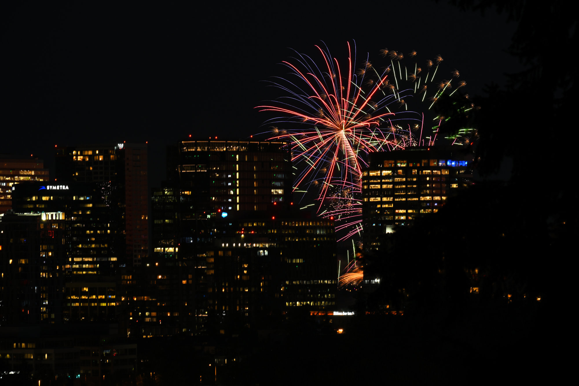
3,0s f/13 ISO 100/21° 50-250mm f/4,5-6,3 VR f=175mm/262mm
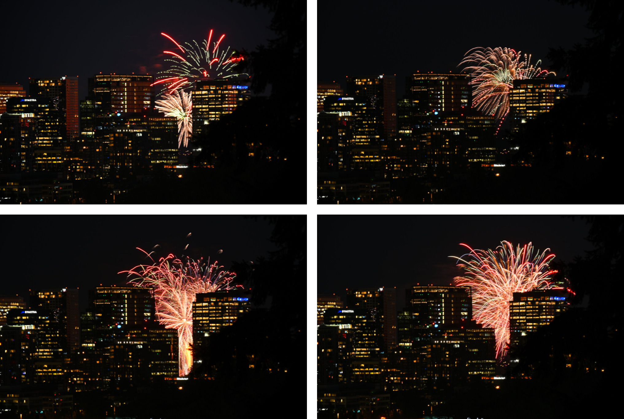
1,3s 4s, 4s, 5s f/13 ISO 100/21° 50-250mm f/4,5-6,3 VR f=175mm/262mm
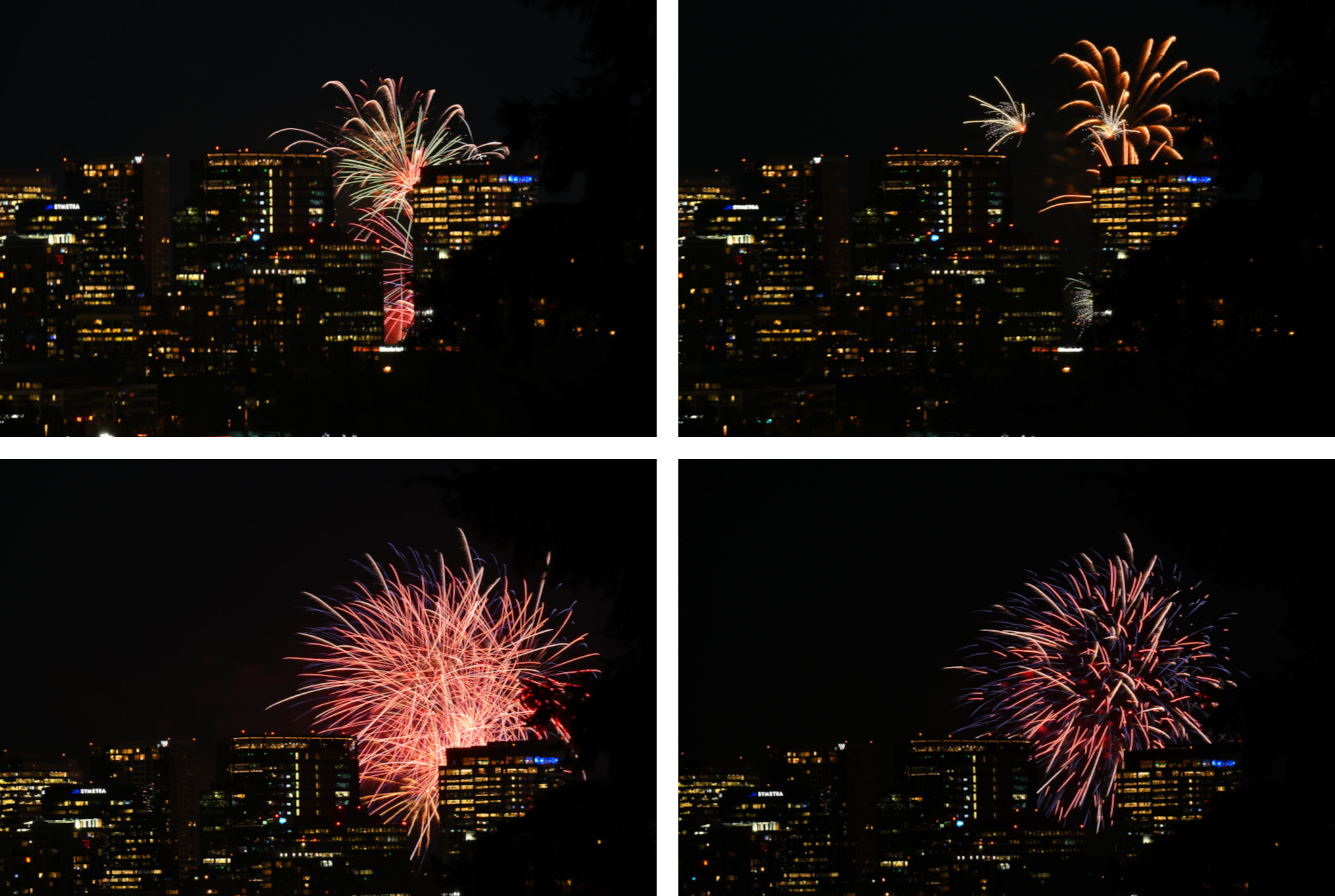
5s 3s 4s 1,6s f/13 ISO 100/21° 50-250mm f/4,5-6,3 VR f=175mm/262m
I have watched over twenty of them. Was only supposed to be here for one.
Actually, it all started with Internet Explorer. That was the reason for the trip. One year, a browser, and then back.
Internet Explorer 4. Internal build. Not available in stores.1
The reason the one-year plan did not end on schedule.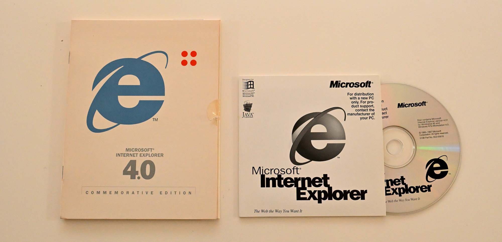
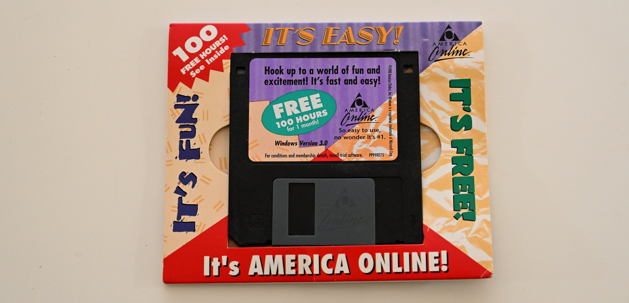
And remember America Online? 100 free hours. At 28.8k, that was about 1.2 GB of theoretical ambition.
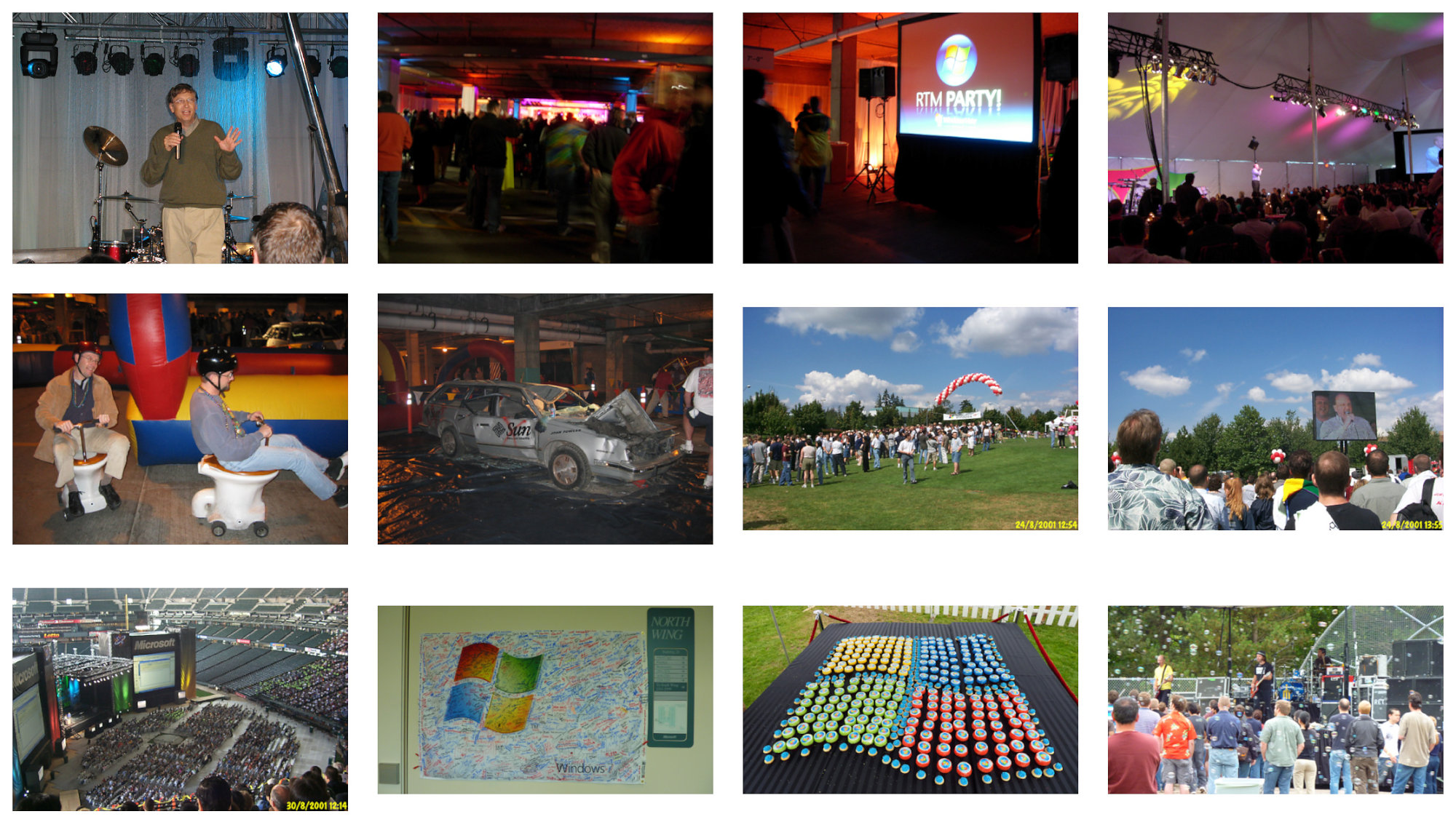
Eventually, there were ship parties.2
Major releases. Major parties.
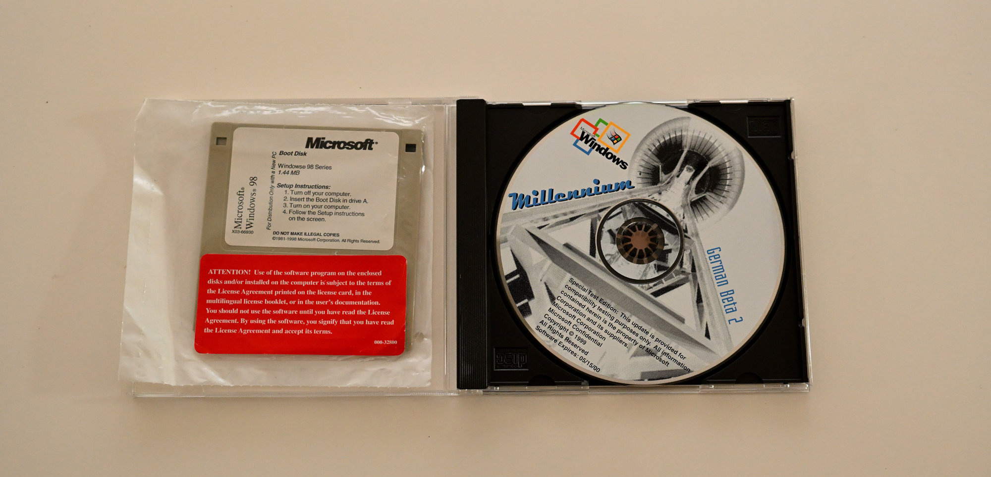
The world kept changing around me. So did the work. The browser became Windows, the one you are probably running right now.
Windows Millennium Edition, Beta 2. The version before the version. Space Needle included.
Still waiting for first boot.
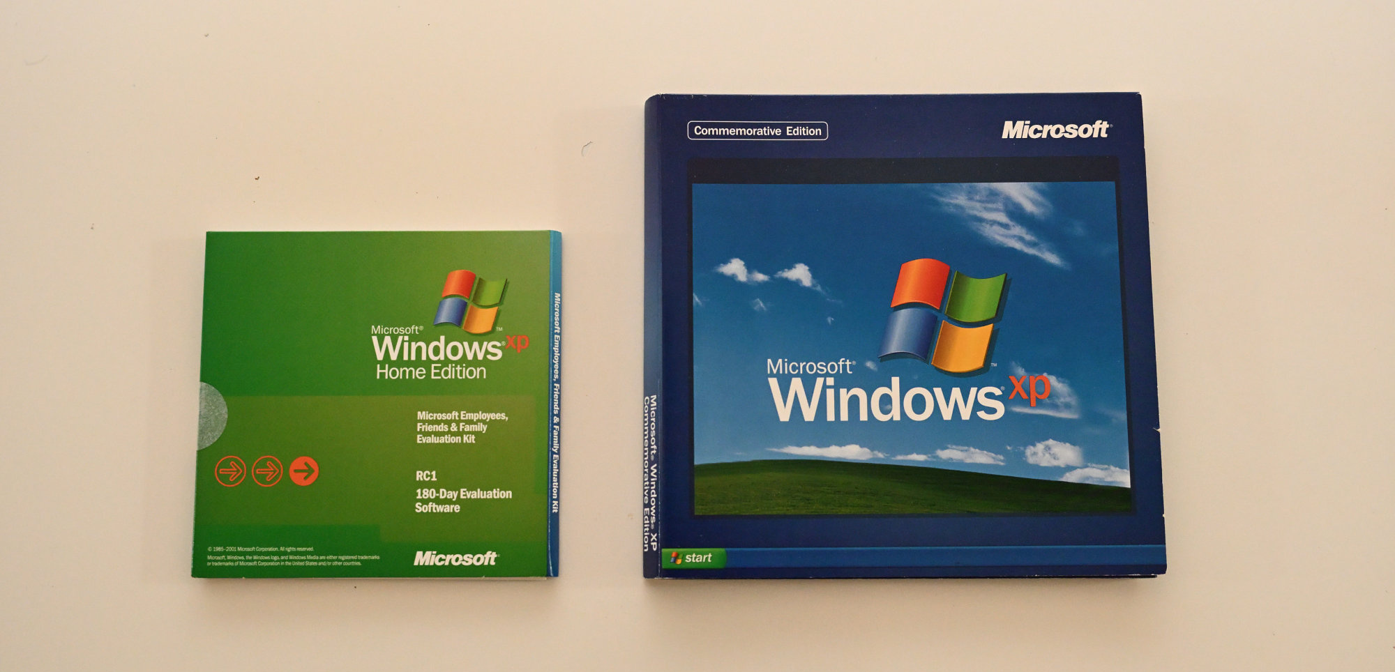
With the credits booklet. One highlight.
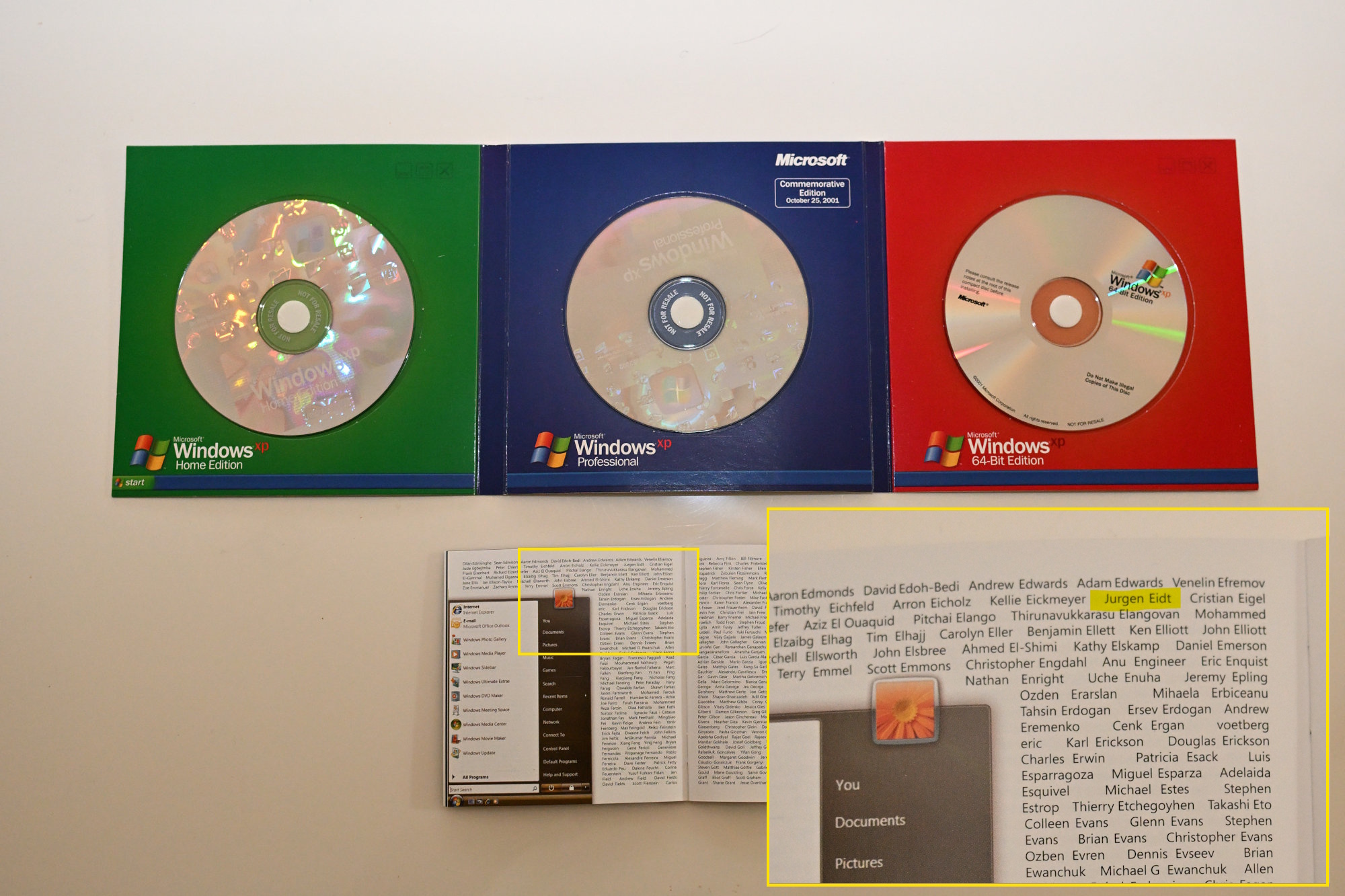
The foundation came first. The thank you came later.
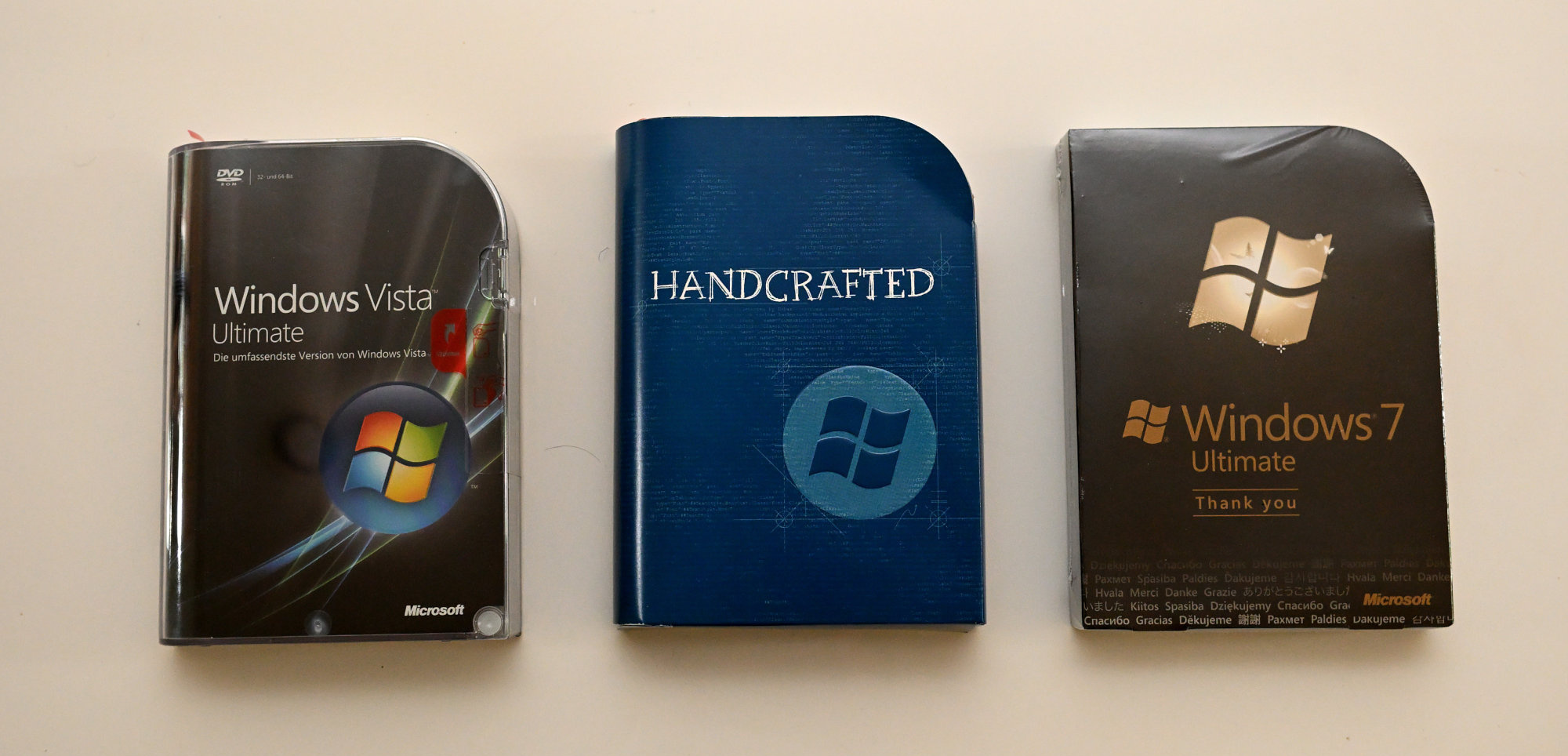
And then AI arrived, and suddenly even the tools had tools. Maybe you asked one something today. That answer has a longer history than it looks.
The sky eventually reclaimed the agenda.
3,0s f/13 ISO 100/21° 50-250mm f/4,5-6,3 VR f=175mm/262mm
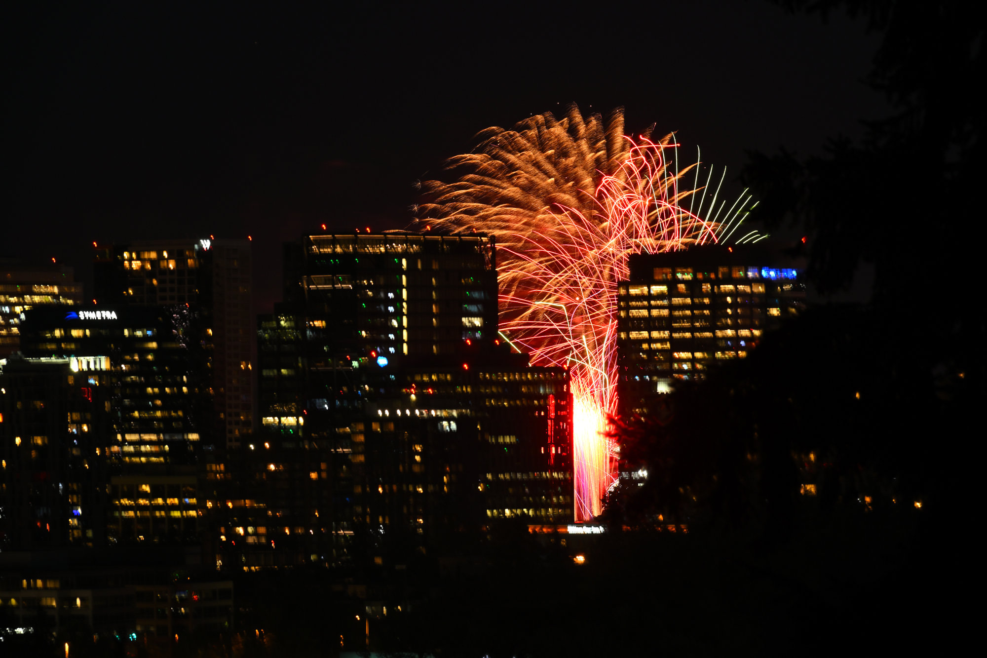
Photographing fireworks is practice in letting go of the plan. The light does what it wants. The camera catches what it can.3
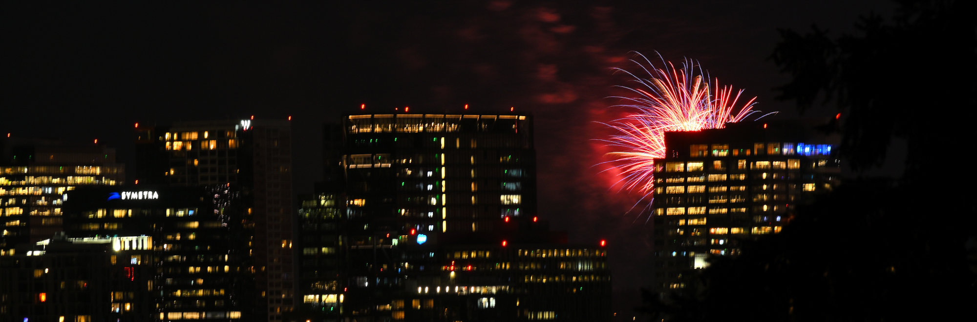
The horizon always narrows, keeping your outlook undimmed. Rarely a moment ends entirely still.
-
Vault inventory was not loaded for this post. Selective deaccessioning is not out of the question. ↩
-
Release parties were the traditional proof that the build had escaped. Bill Gates is standing almost directly in front of me, making an announcement. I talked with him later. Another frame has Steve Ballmer on stage, doing exactly what you would expect. The 1990s were not subtle. ↩
-
Practical notes are here: Photographing Fireworks at a Distance 🎆. At 175 mm, even a tripod notices footsteps. ↩
-
-
June Solstice Moon 🔭🌓
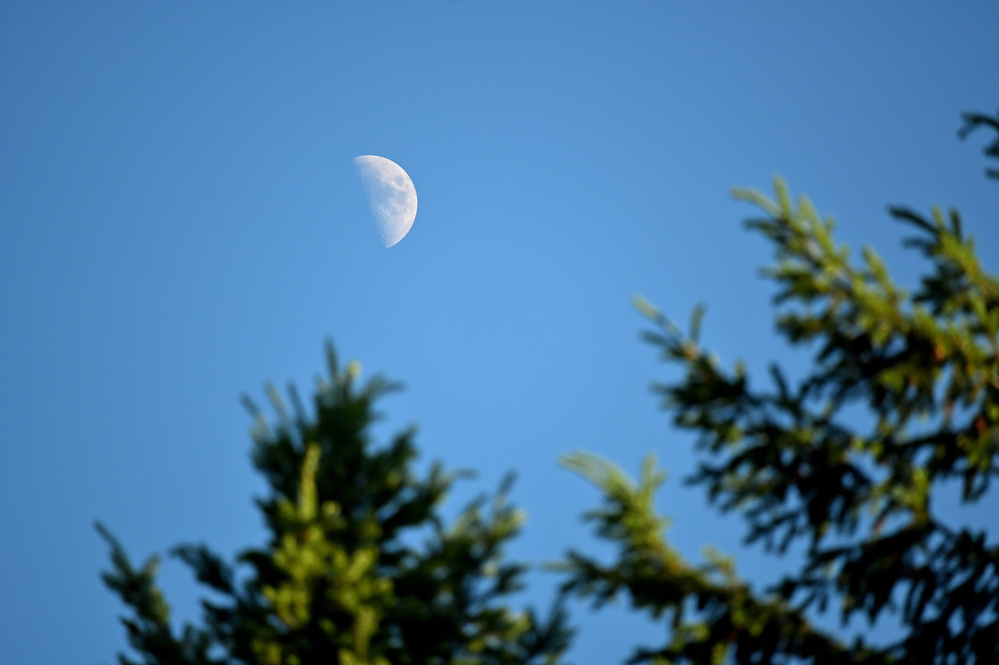
June 21st, 2026, 19:194. Summer solstice: the Sun reached its northern limit, the day stretched as far as it could, and the Moon was already visible in the blue evening sky.
The day was clearly not finished. The sky was still blue, the trees were still in sunlight, and the Moon had already arrived.
Not bright enough to take over, not faint enough to ignore. Just early.
Another moon sighting. No agents on duty this time, but the sky was clearly being monitored: Zunehmender Halbmond 🌓🌛.
Taken handheld with my Z50 and the NIKKOR Z DX 50-250 mm 1:4,5-6,3 VR. The tripod stayed inside.
1/500s f/6,3 ISO 250/25° 50-250mm f/4,5-6,3 VR f=250mm/375mm
The second image is a crop from the original 5568 × 3712 photo. The crop is 1015 × 677 pixels.
The lens was at 250 mm on a Nikon Z50. With the 1.5× APS-C crop factor, the EXIF reports this as 375 mm in 35 mm equivalent terms.
The additional digital crop factor can be calculated from the diagonal ratio:
$$ c_\text{digital} = \frac{\sqrt{5568^2 + 3712^2}} {\sqrt{1015^2 + 677^2}} $$
$$ c_\text{digital} = \frac{6692}{1220} \approx 5.49 $$
So the cropped image has an effective 35mm-equivalent focal length of:
$$ f_\text{eq,crop} = 250\,\text{mm} \times 1.5 \times 5.49 $$
$$ f_\text{eq,crop} \approx 2057\,\text{mm} $$
Or, starting from the EXIF equivalent focal length:
$$ 375\,\text{mm} \times 5.49 \approx 2057\,\text{mm} $$
In framing terms, the result is about 2050 mm full-frame equivalent.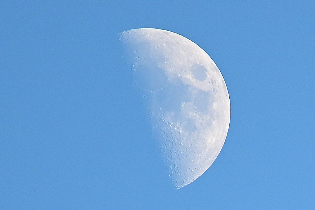
It started as 250 mm and ended up at 2050 mm. With one more zero and some cropping, the Z50 became a small handheld observatory for one evening.
-
19:19 is photo time. The solstice itself had already occurred at 01:24, when the Sun reached its northernmost declination and began its slow return south. ↩
-
-
Bellevue Piloti-Skulptur
Piloti is an ultra-thin, self-supported aluminum rotunda by Marc Fornes / THEVERYMANY, commissioned by the City of Bellevue. It stands at the edge of Downtown Park, close to the towers but clearly not designed to think in straight lines. The trees help. So does the sunshine.
It is one of those places where I stop longer than planned.
1/1000s ISO 100/21° f=7,5mm
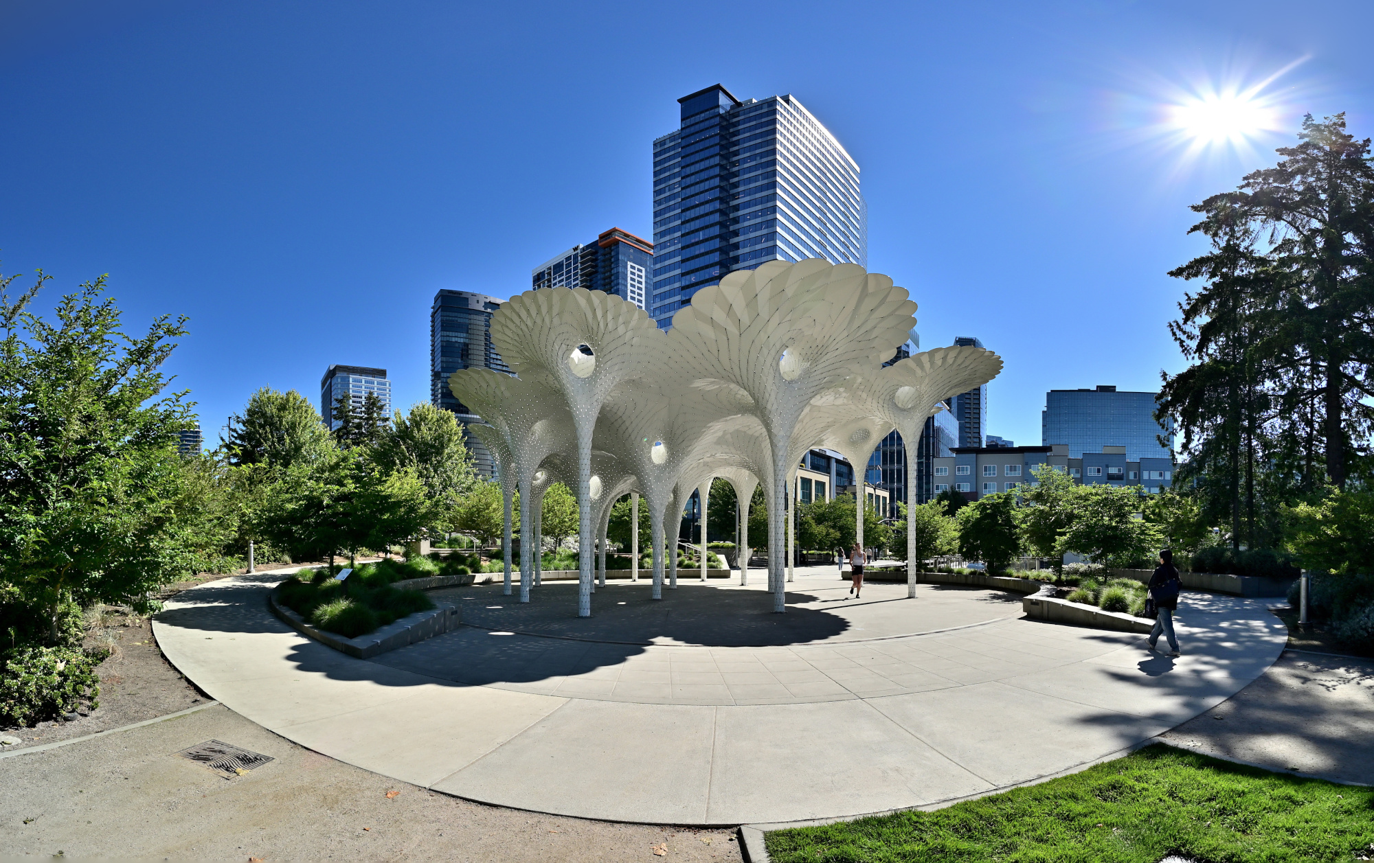
The sun was bright enough to make every shadow look like it had been organized in advance.
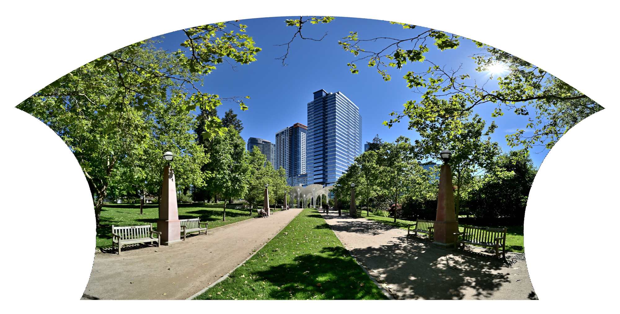
1/1000s ISO 100/21° f=7,5mm
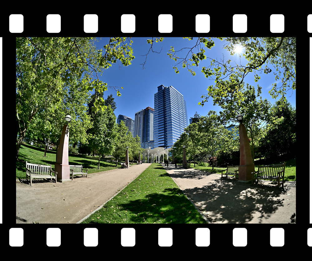
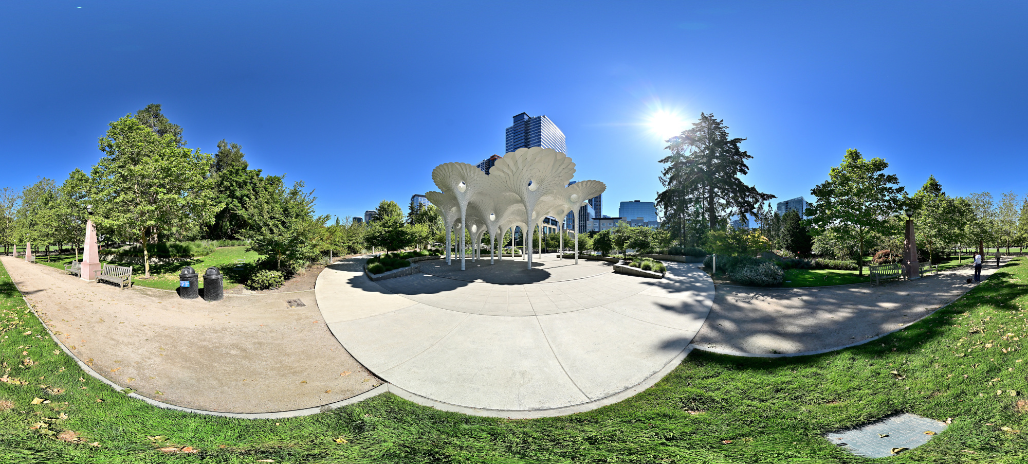
The theme for The World Wide Panorama was Exception, and this was the view that made the whole series happen. Bellevue around Piloti is all glass, clean edges, and corporate geometry. Downtown edges met one deliberate anomaly, yet the city kept its face straight. Then this thing stands there, soft and strange, like it grew overnight and nobody wanted to ask too many questions.
That was the exception I wanted: not a spectacle, but something that quietly refuses to behave like the city around it.
Interactive Panorama Piloti-Skulptur 1 360x180
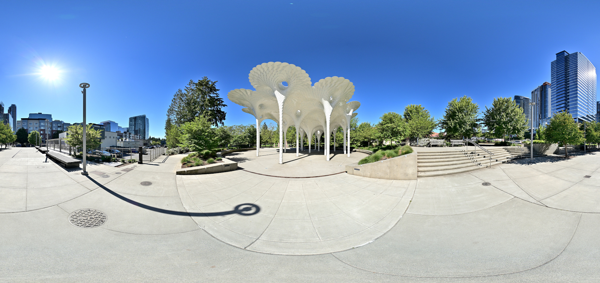
1/1000s f/5,6 ISO 100/21° f=7,5mm
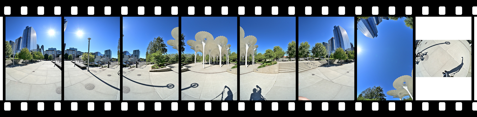
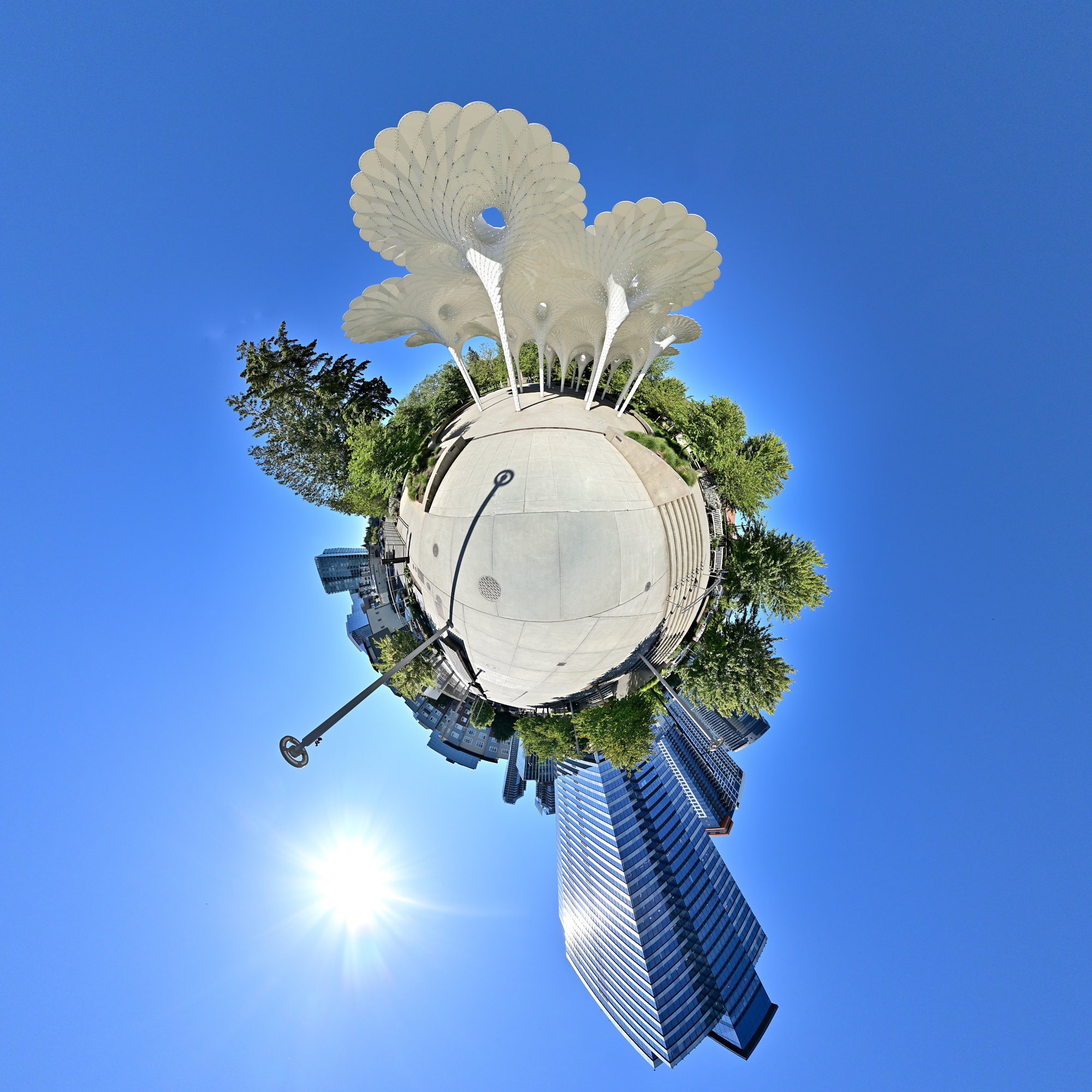
The Panorama Supervision Unit also made a brief appearance.5
From this side, Piloti feels less like a landmark and more like something the park quietly kept for itself.
Interactive Panorama Piloti-Skulptur 2 360x180
1/1000s f/5,6 ISO 100/21° f=7,5mm
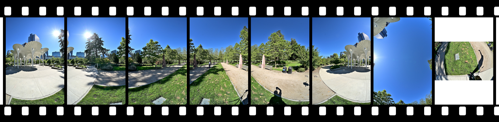
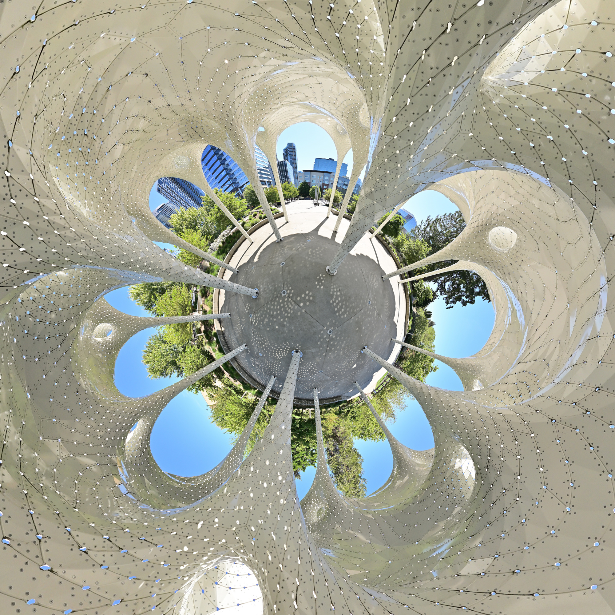
The little planet version gives the park a suspicious amount of authority.
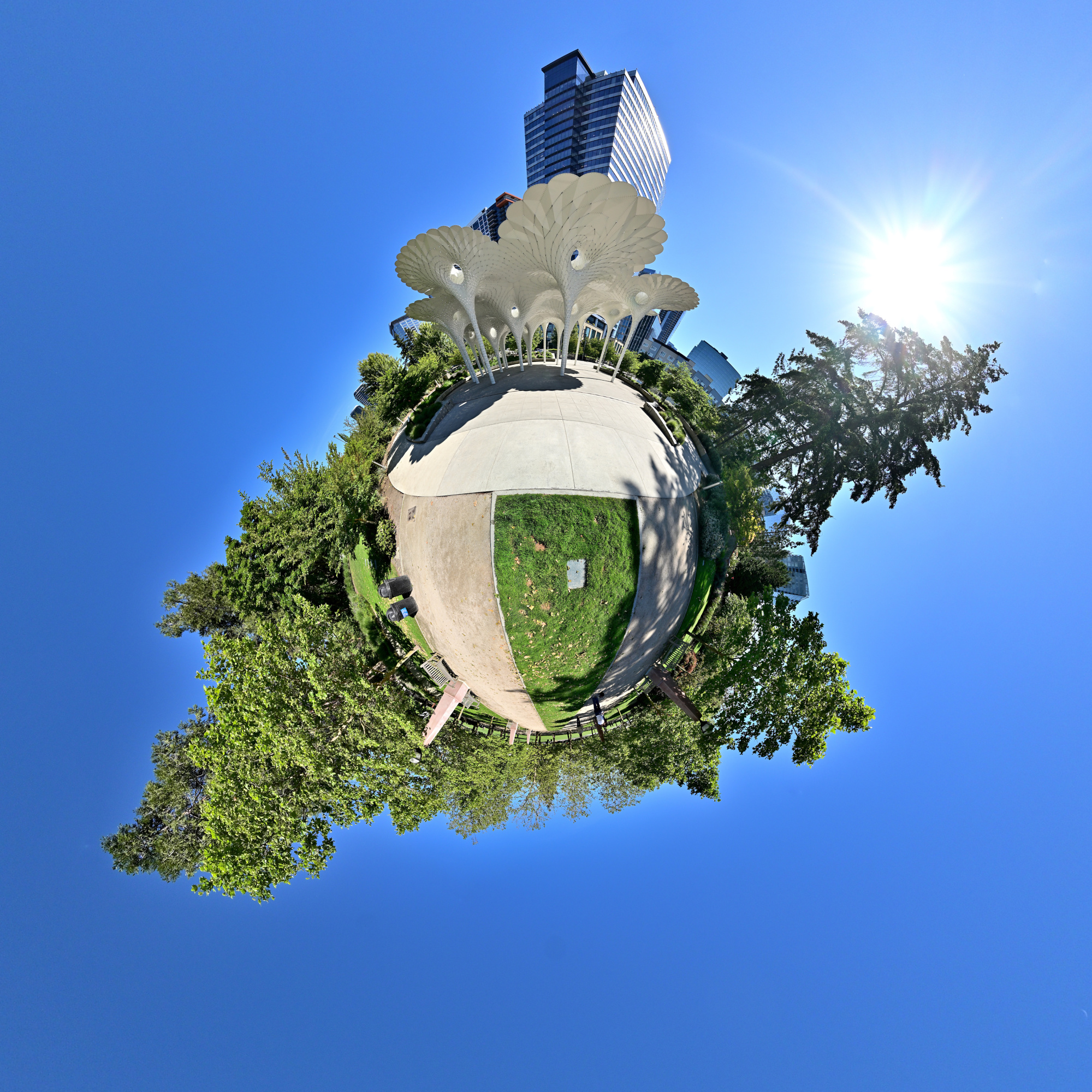
Inside, it feels less like looking at the sculpture and more like standing under its idea.
Interactive Panorama Piloti-Skulptur 3 360x180
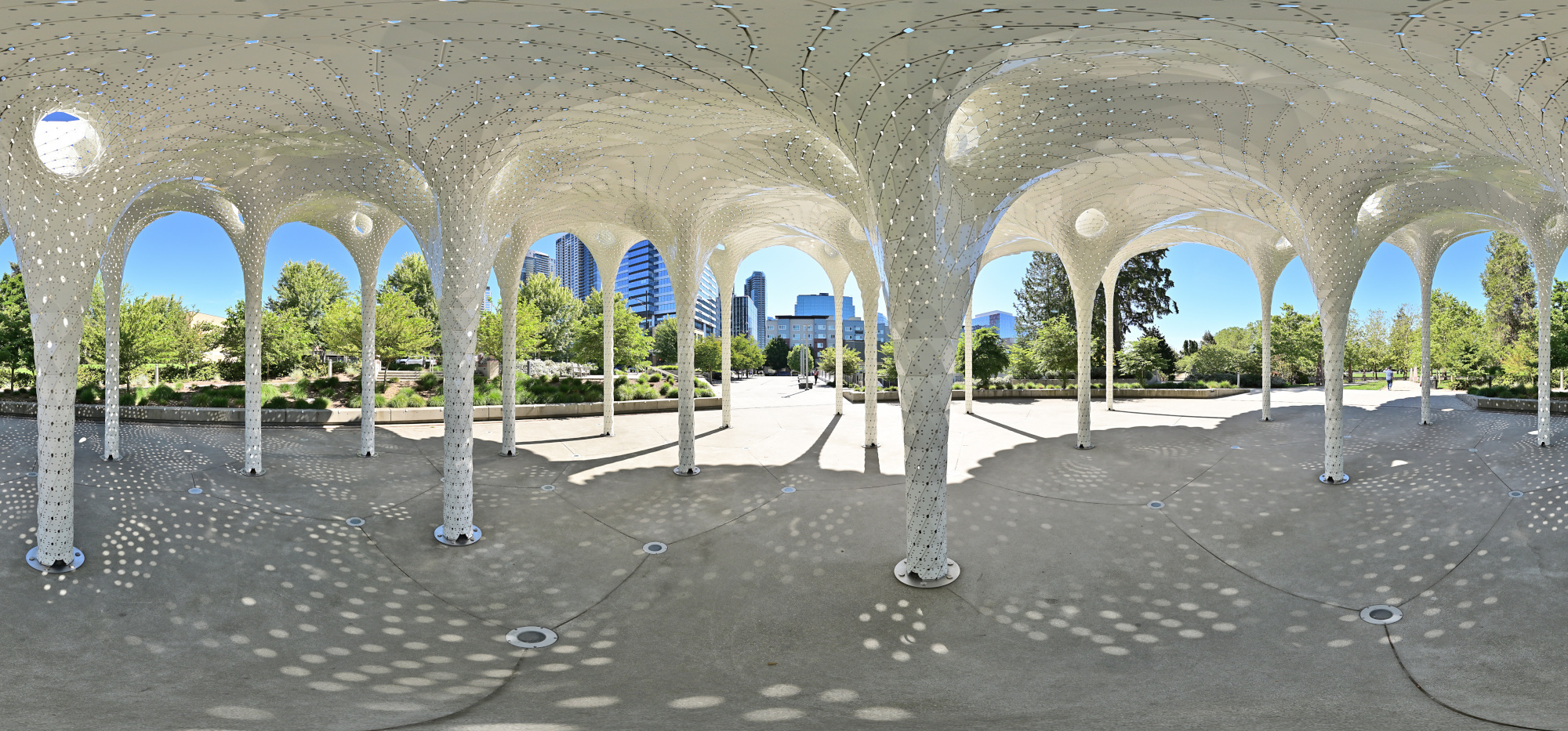
1/640s f/5,6 ISO 100/21° f=7,5mm
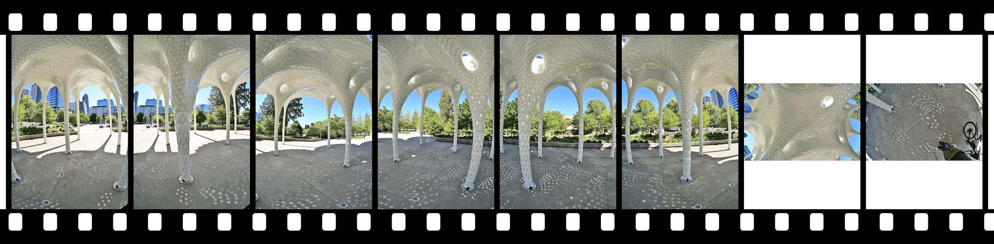
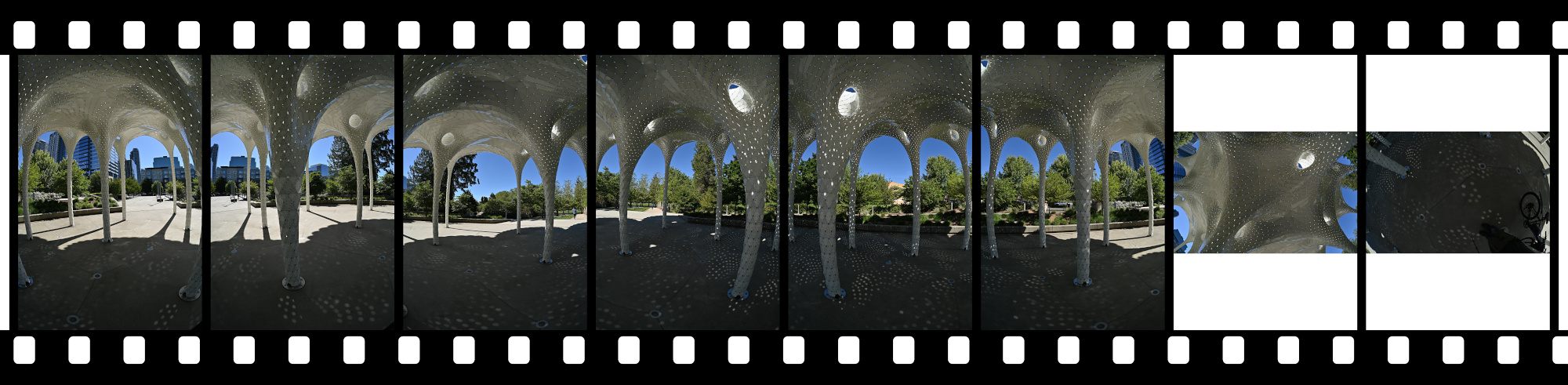
These are the original NEF frames; with the hard contrast under the sculpture, the RAW data was useful for recovering highlight and shadow detail and building a more natural HDR-like result.
The last little planet makes a tiny roofed world out of it. No permit required.
-
After previous observations by Agent Gull and Agent Ducky, the Panorama Supervision Unit opened another file in the city park.
Agent Crow with the Peanut-Cam
First contact was made by a crow carrying a small peanut-shaped device, later classified as a field camera of the Panorama Supervision Unit.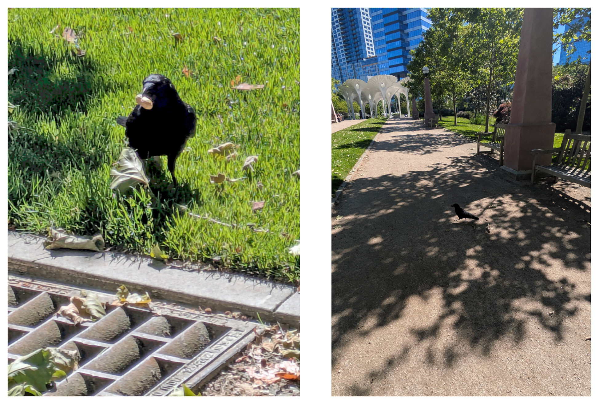
Ground Inspection
Agent Crow returned without visible equipment and stopped on the path, continuing the close-range panorama check under ordinary park conditions.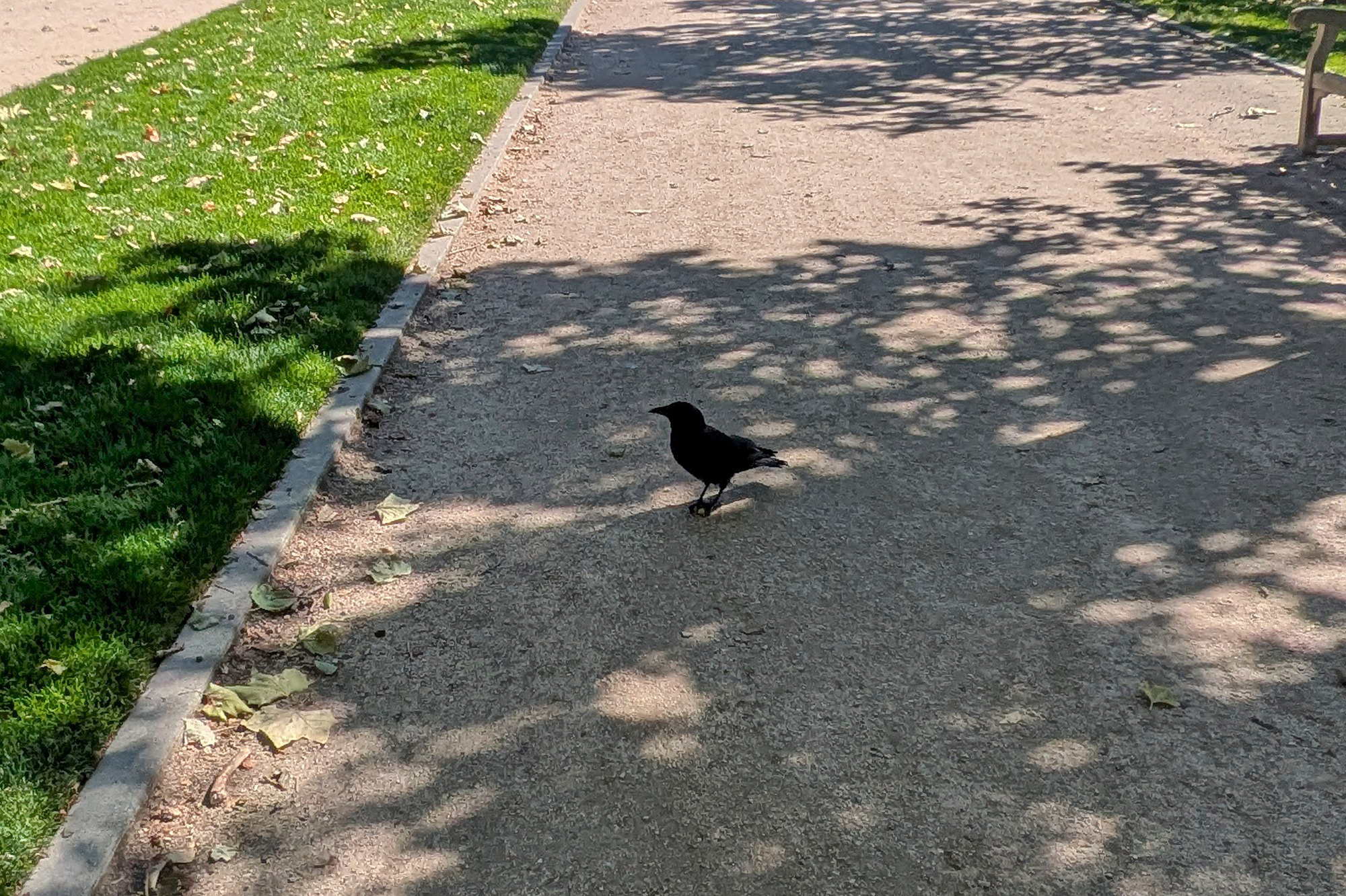
Following the Route
The inspection continued along the path with the calm certainty of someone who had already received instructions.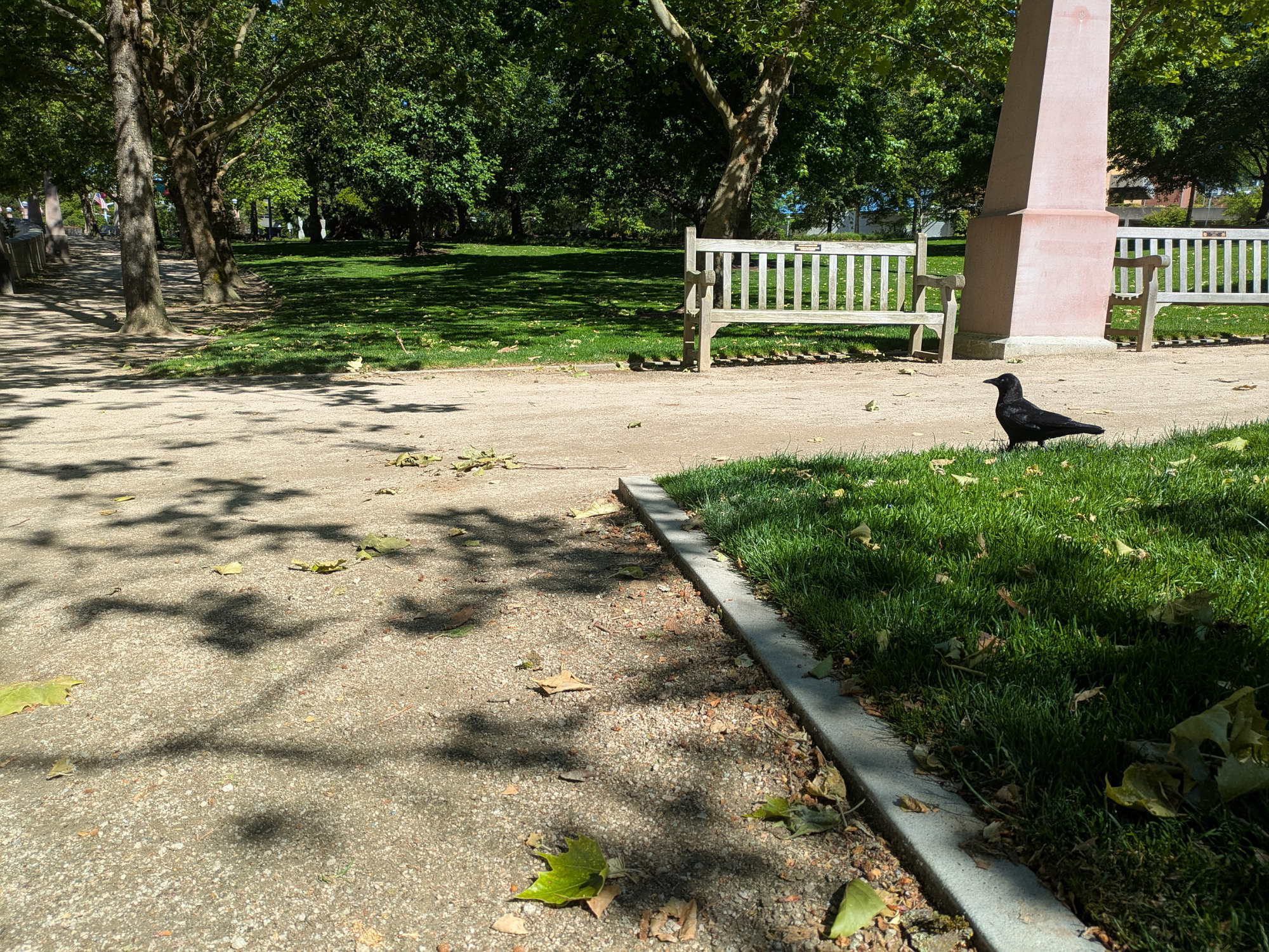
Aerial Departure
Shortly after that, Agent Crow left by air.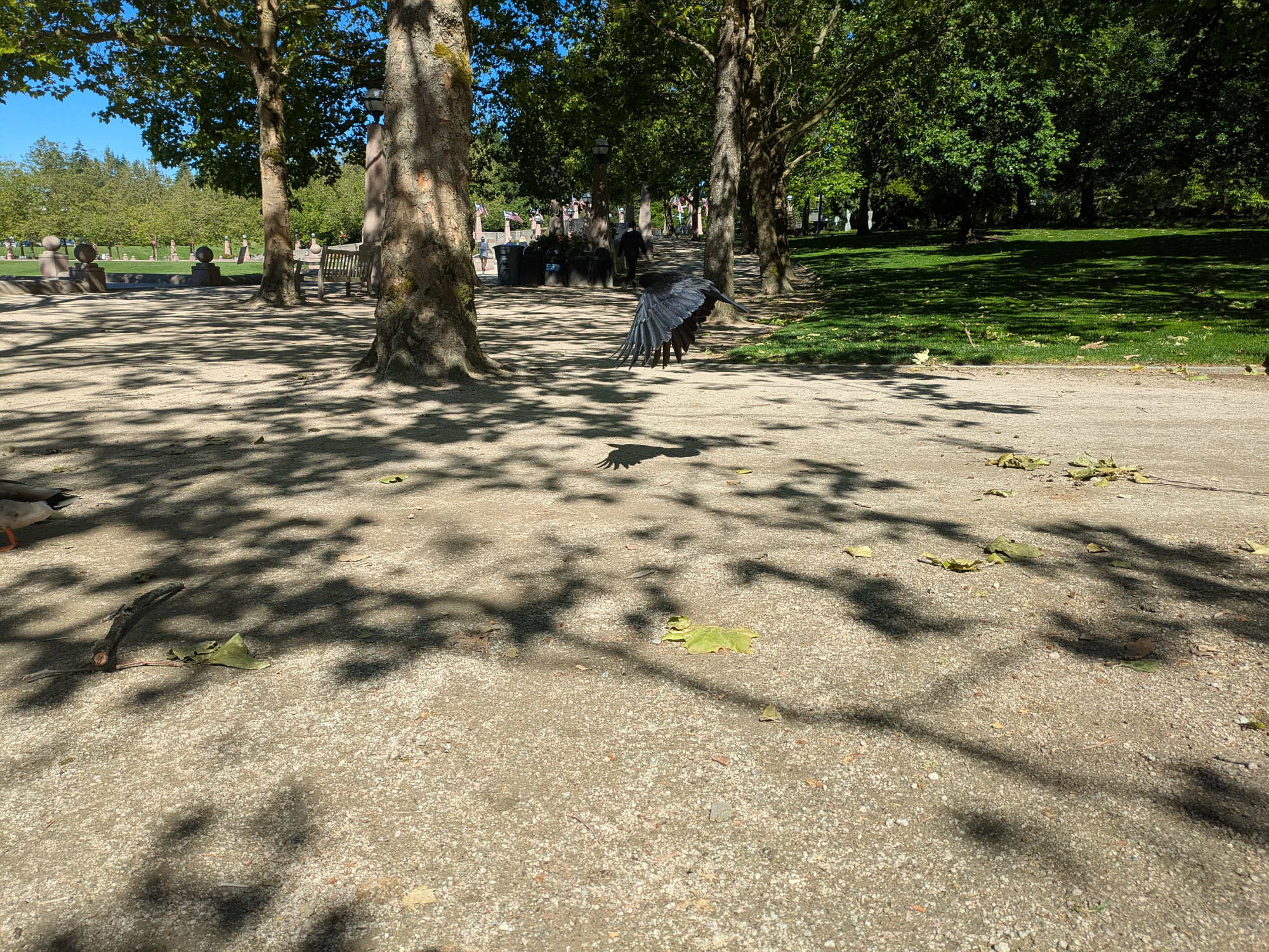
Agent Toni and Agent Tini
The file was then handed to a two-agent operation. Agent Toni and Agent Tini arrived together and performed a silent double check of the panorama perimeter.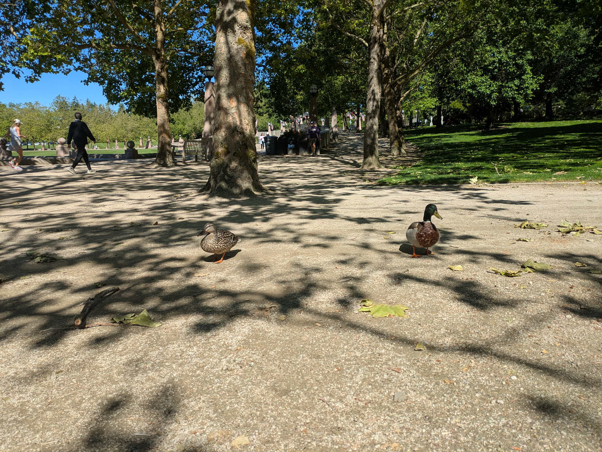
The Panorama Supervision Unit recorded the visit; all panorama activity remains under quiet observation.
↩
-
-
MCP Resources: The Quiet Half of the Protocol
Most MCP examples start with tools.
That makes sense. Tools are easy to demonstrate: the model asks, the server does something, and a result comes back.
Resources are quieter. They do not run an action. They expose named read access to state.
That distinction is the point.
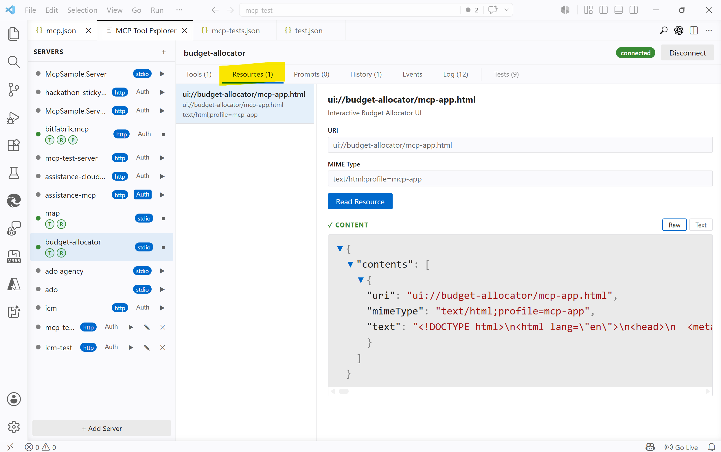
The screenshots show MCP Tool Explorer connected to the MCP SDK example server
@modelcontextprotocol/server-budget-allocator.
Tools Are Commands
A tool is a command exposed by an MCP server.
It might calculate something, start a build, create an issue, query a database, send a message, rotate an image, or trigger a deployment. A tool has input, behavior, and a result. Sometimes it also has side effects.
That is why tool calls are the easy part of MCP to explain. They look familiar. The model asks for an operation, the host calls the server, the server replies.
tools/call run_tests
  input:  { "suite": "unit" }
  output: { "passed": 128, "failed": 0 }
Good tools should be explicit. They should have clear names, clear schemas, and clear errors. If a tool changes the world, that should not be hidden behind a vague description.
So far, so normal.
Resources Are Named Reads
A resource is different.
A resource is not a command. It is a URI the client can read from the server.
resources/list
  build://latest/log
  build://latest/summary
  config://current
  trace://last-run
  device://temperature
The server owns those names. It decides what exists, what each URI means, and what content is returned when the client calls
resources/read.That content may come from a file. It may come from memory. It may be assembled from an API call, a database row, a device sensor, a log tail, or a generated summary. The important part is not where the bytes come from. The important part is that the operation is a read.
Client -> Server: resources/read build://latest/log
Server -> Client: text/plain content
A resource can be dynamic and still be a resource.
metrics://nowmight be different every time it is read.build://latest/logmight point to whatever the latest build produced.device://temperaturemight be sampled live.Dynamic does not mean action. It means the read is resolved at request time.
For example, a test server might expose a
live-statusresource. Reading it can return the server's current uptime, request counters, active configuration, or last activity. The values may change every few seconds, but the protocol shape stays the same: the client reads named state from the server.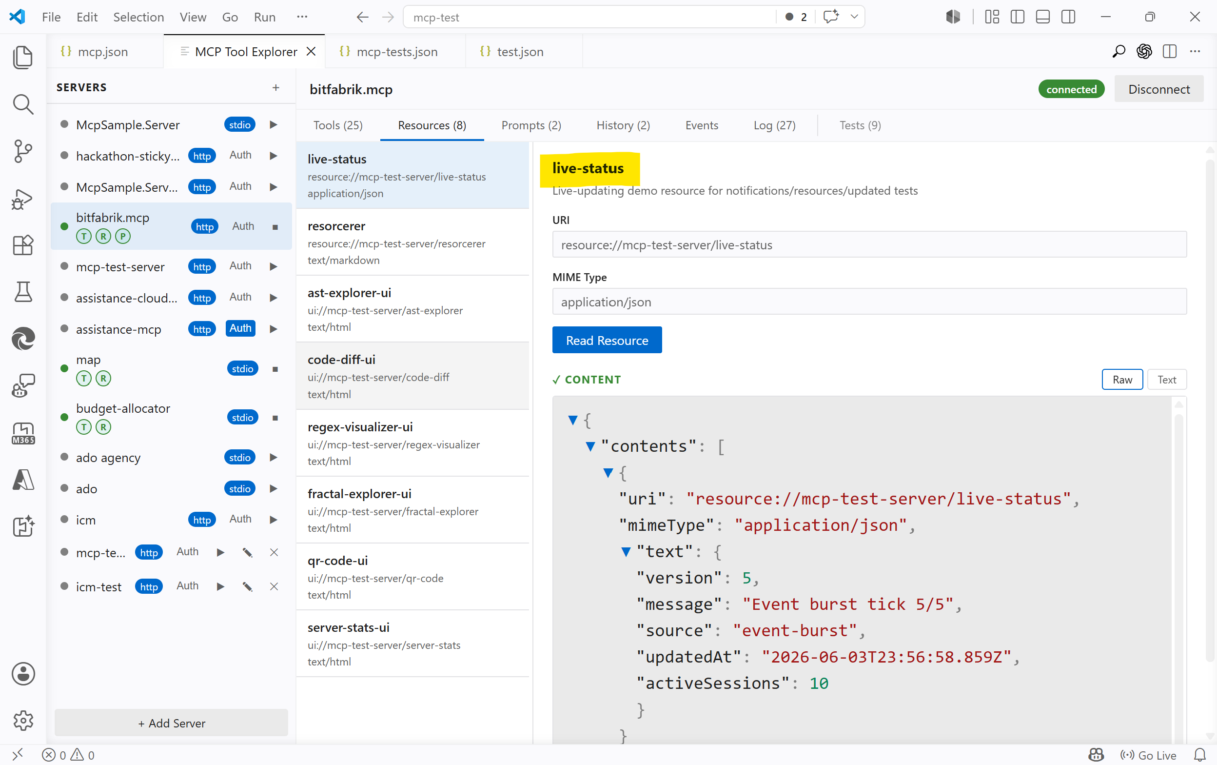
Another good example is MCP Apps. In that case, a tool can point at a
ui://resource. The client reads that resource, receives an HTML document, and renders it as the app UI. The resource is not just metadata around the tool; it is the thing that implements the interactive surface.That still follows the same rule: the app HTML is fetched through
resources/read. The tool may trigger the experience, but the UI itself is loaded as a named read from the server.I wrote about the full app mechanism, sandboxing, protocol flow, and host implementation in MCP Tool Explorer Supports MCP Apps: Protocol, Code, and the Fine Print.
The Model Does Not See Resources Automatically
This is the part that is easy to get subtly wrong.
Resources are not hidden context that the model magically knows about. They are server-side readable state with names.
The client can list resources and read them from the server. It does not need to know where the data lives or how it is collected. For a log resource, the client does not know the logs. The server does. The client only knows that a named read is available.
After reading a resource, the client can show the returned content to the user, cache it, use it internally, or include selected contents in a model request. But the model only sees the resource if the client deliberately includes that returned content.
Until then, the resource is available to the client, not present in the model context.
That is why the resource boundary matters. The server exposes knowledge the client does not otherwise have: logs, status, snapshots, generated reports, files, device state, or app HTML. A resource has an owner, a URI, a MIME type, a lifecycle, and a read boundary. The server says what can be read; the client asks for it by name.
That explicit boundary is what makes the system easier to inspect and reason about.
A Small Example
A server could expose a build system like this:
resources/list
  build://latest/summary
  build://latest/log
  build://latest/artifacts

tools/list
  run_build
  run_tests
  deploy_preview
The resources describe current state. The tools perform operations.
A client might first read
build://latest/summaryand show it to the user. If the model needs more detail, the client can readbuild://latest/logand pass only the relevant part into the next request. If the user asks for a new build, the client callsrun_build.After that, the server may update what
build://latest/summaryreturns. It may also notify the client that the resource list or resource contents changed, depending on the server and host behavior.The important thing is that reading the log and starting the build are separate protocol concepts.
One observes state. The other asks for work.
Resource Design Is API Design
The hard part is not implementing
resources/read. The hard part is deciding what deserves a URI.A good resource should be specific enough to be useful, but not so tiny that the client has to stitch together a hundred fragments. It should be stable enough to reference, but not so broad that every read becomes a data dump.
There are practical questions:
- How current does the data need to be?
- Can the client cache it?
- Who is allowed to read it?
- Does it contain secrets?
- Should large content be summarized or paged?
- Is this really a read, or is it a tool pretending to be harmless?
That last one matters.
Reading
build://latest/logis a resource. Starting a build is a tool.Reading
config://currentis a resource. Changing the config is a tool.Reading
device://temperatureis a resource. Turning on a relay is a tool.The names are not decoration. They define where the read boundary is.
Why This Matters
MCP is often described as a way to give models tools. That is true, but incomplete.
Tools expose commands. Resources expose readable state.
That separation gives MCP clients a cleaner way to work with systems that have more going on than one request and one response. Logs can be read without starting anything. Current configuration can be inspected without changing it. A server can expose status without turning every status check into a tool call.
It also helps humans. A resource list is inspectable. A resource URI can be logged. A resource read can be replayed. Permissions can be reasoned about at the boundary between "may read this" and "may do this".
That is less spectacular than a flashy agent demo.
It is also closer to how real software survives contact with Tuesday.
The Short Version
A tool is a command.
A resource is a named read.
The model does not automatically have either one. The MCP client connects to the server, discovers what the server exposes, and can then call tools or read resources by name.
That may sound like a small protocol detail. It is not.
It is the difference between assuming the client already knows the state and giving it a clean way to ask the server what the server knows.
-
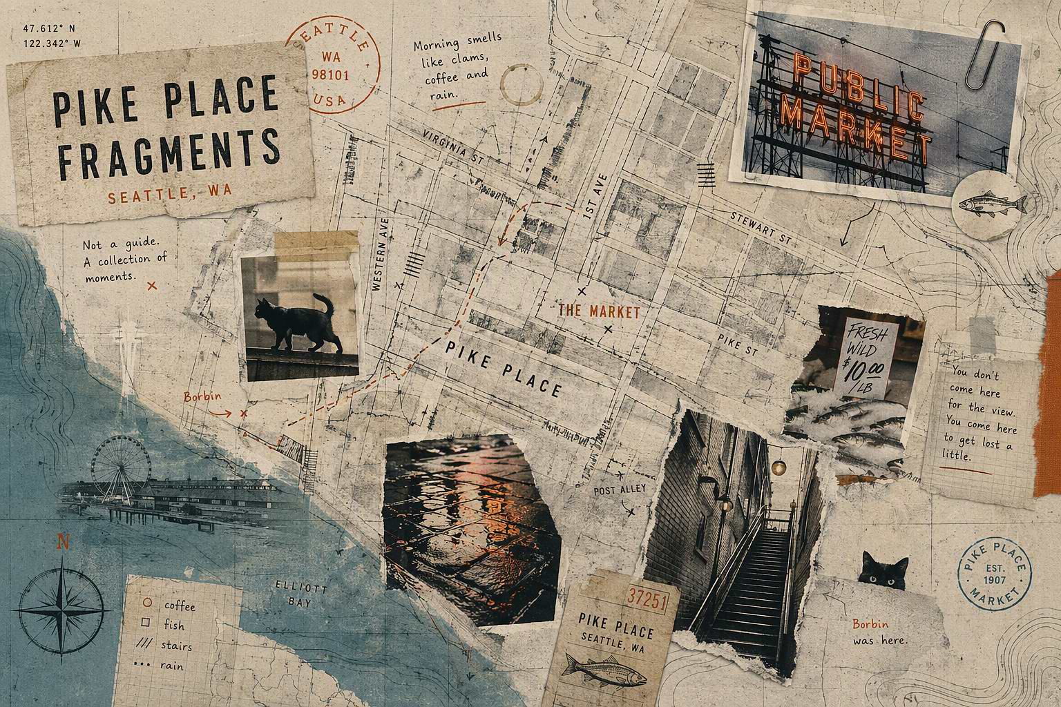
Pike Place Fragments
On a bright Seattle day, Pike Place Market is every bit the postcard, but it keeps opening up in other directions too. The familiar sights are still there, of course, but the place also pulls toward the water, into side streets, through shop windows, and into small moments that are easy to miss. Somewhere between stairs, neon reflections, fish crates and narrow alleys, Pike Place slowly turns into something larger than its landmarks. These photos are a walk through those other sides of Pike Place, with good weather doing more than its fair share of the work.
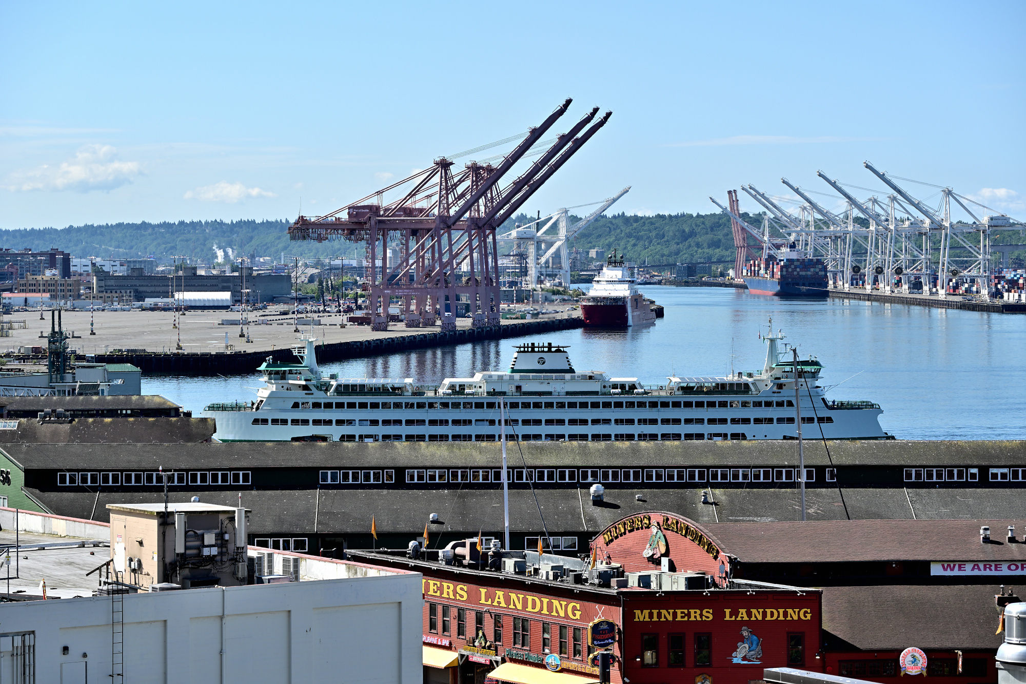
Before the market takes over, the waterfront has already started the conversation.
Sunshine, harbor cranes, and a ferry coming in from the Sound: Seattle starts the day looking busy.
1/400s f/7,1 ISO 100/21° 18-140mm f/3,5-6,3 VR f=68mm/102mm
Puget Sound looks almost too relaxed here, considering how quickly the market picks up speed. From City View Park, this is also where Seattle lines up for its city views and panoramas.
1/640s f/6,3 ISO 100/21° 18-140mm f/3,5-6,3 VR f=140mm/210mm
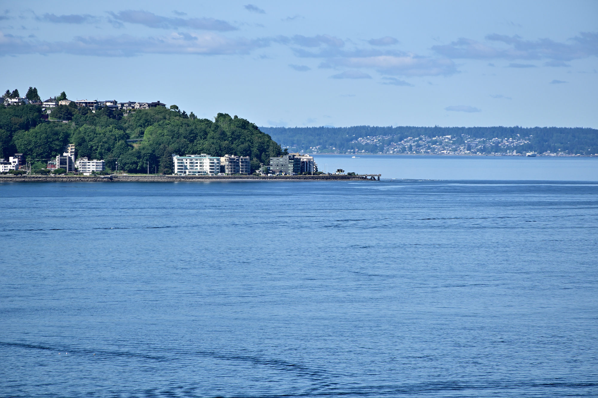
A quiet stretch of blue, while the city keeps refusing to pause.
1/500s f/10 ISO 200/24° 18-140mm f/3,5-6,3 VR f=140mm/210mm
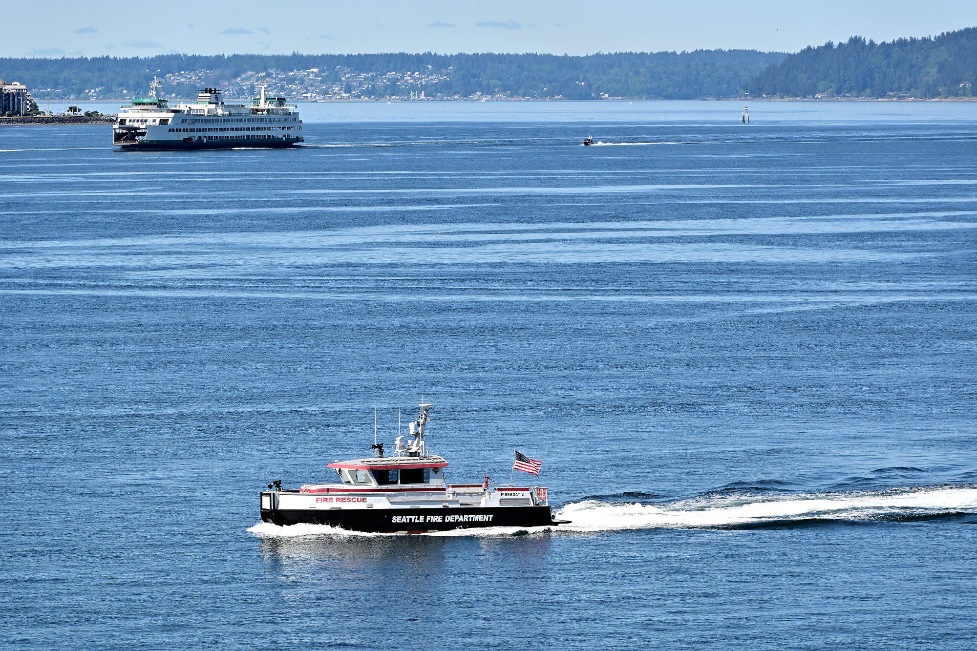
On the waterfront, something is always moving.
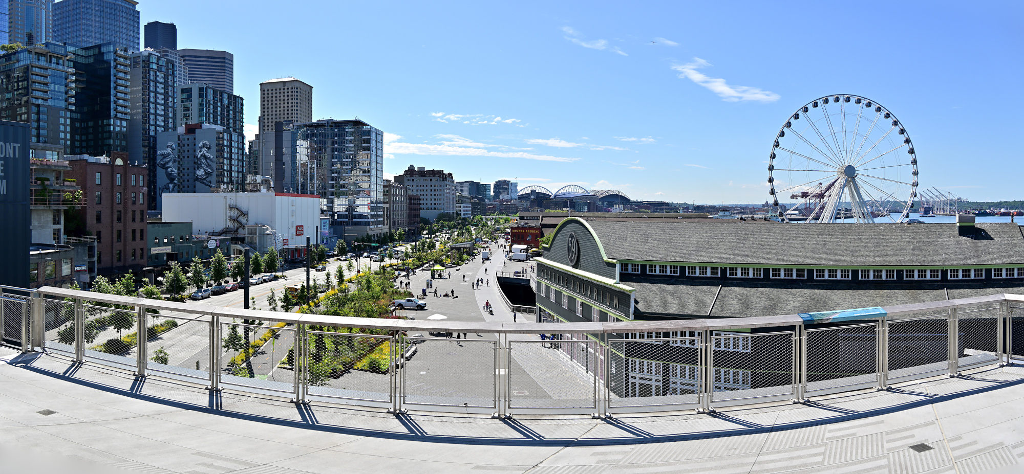
1/400s f/7,1 ISO 100/21° 18-140mm f/3,5-6,3 VR f=18mm/27mm
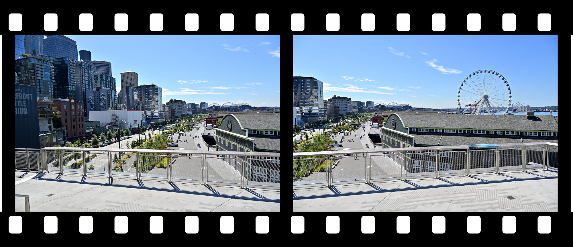
A closer look at the waterfront before the market takes over again.
1/400s f/7,1 ISO 100/21° 18-140mm f/3,5-6,3 VR f=70mm/105mm
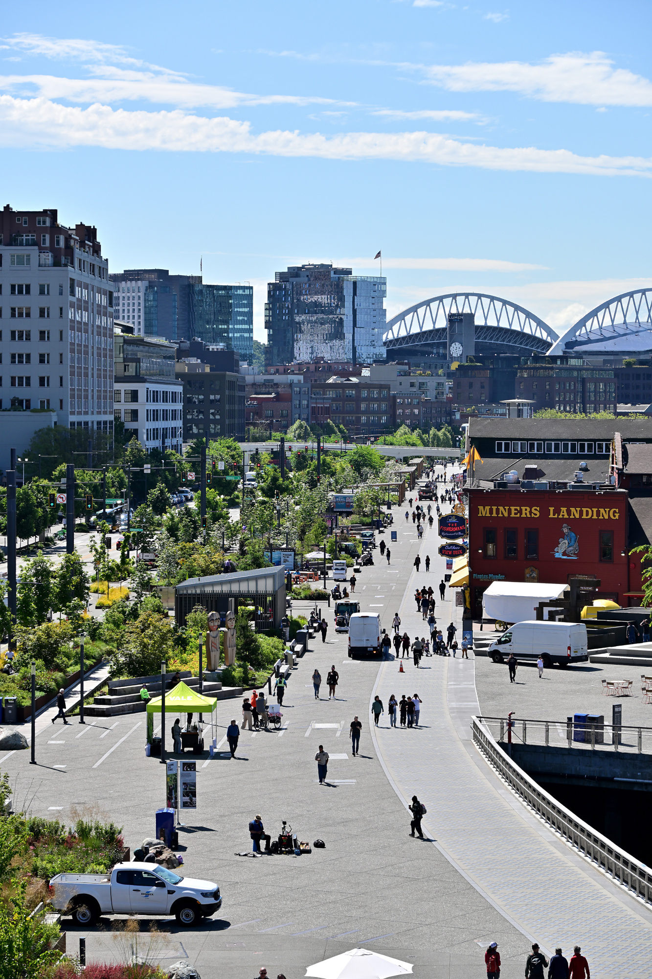
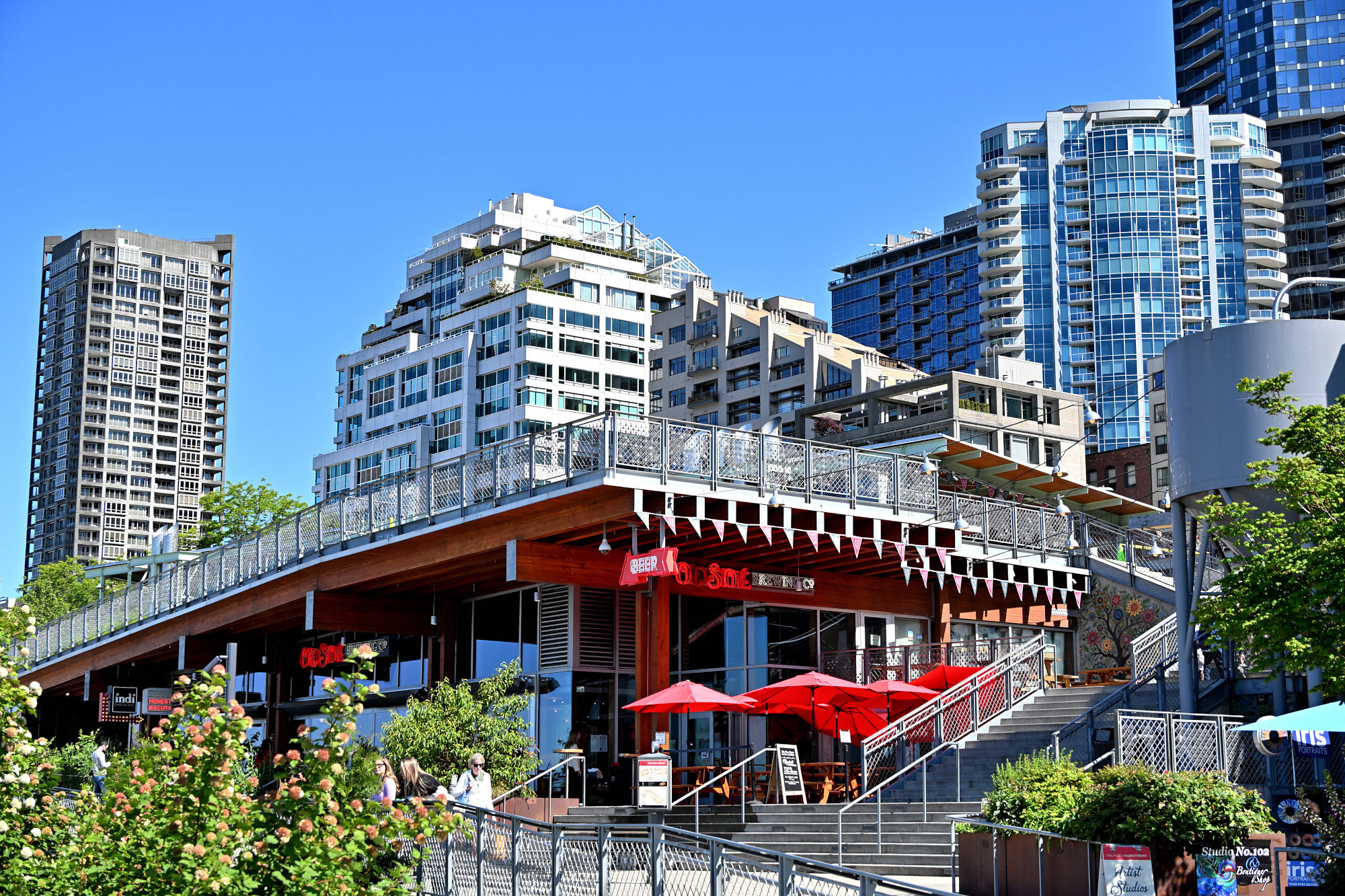
The market edge is all stairs, rails, rooftops, and the promise of something around the corner.
1/320s f/6,3 ISO 100/21° 18-140mm f/3,5-6,3 VR f=35mm/52mm
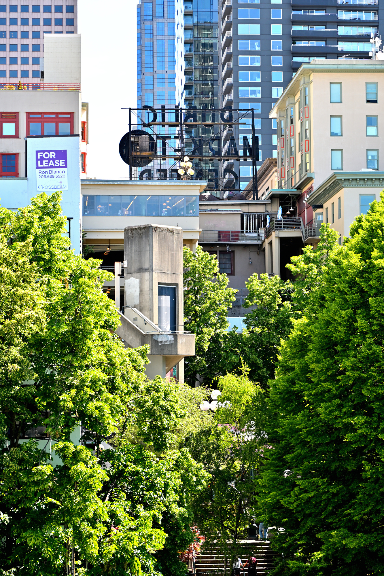
The famous red sign, seen from behind, still knows exactly how famous it is.
1/250s f/5,6 ISO 160/23° 18-140mm f/3,5-6,3 VR f=61mm/91mm
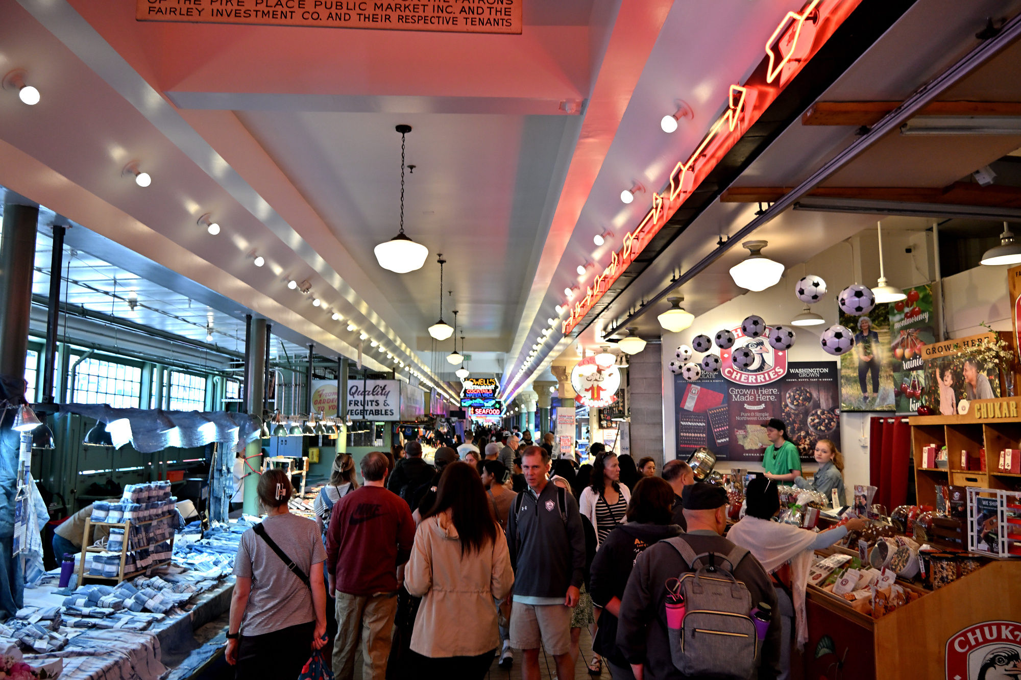
Inside the market, everything gets closer, brighter, and slightly less interested in personal space.
Inside, the market becomes a moving mix of lights, signs, and people with somewhere to be.
1/125s f/3,5 ISO 900 18-140mm f/3,5-6,3 VR f=18mm/27mm
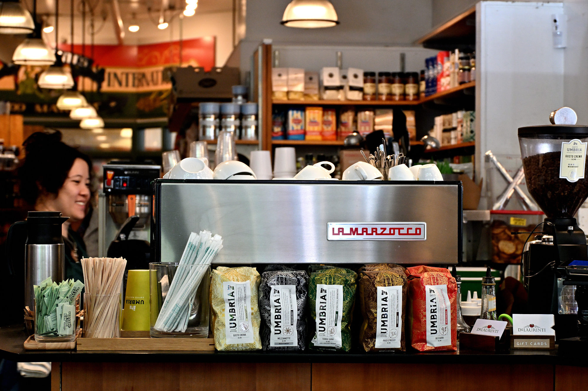
Coffee appears here less as a beverage and more as a basic Seattle utility.
1/125s f/5 ISO 1600/33° 18-140mm f/3,5-6,3 VR f=57mm/85mm
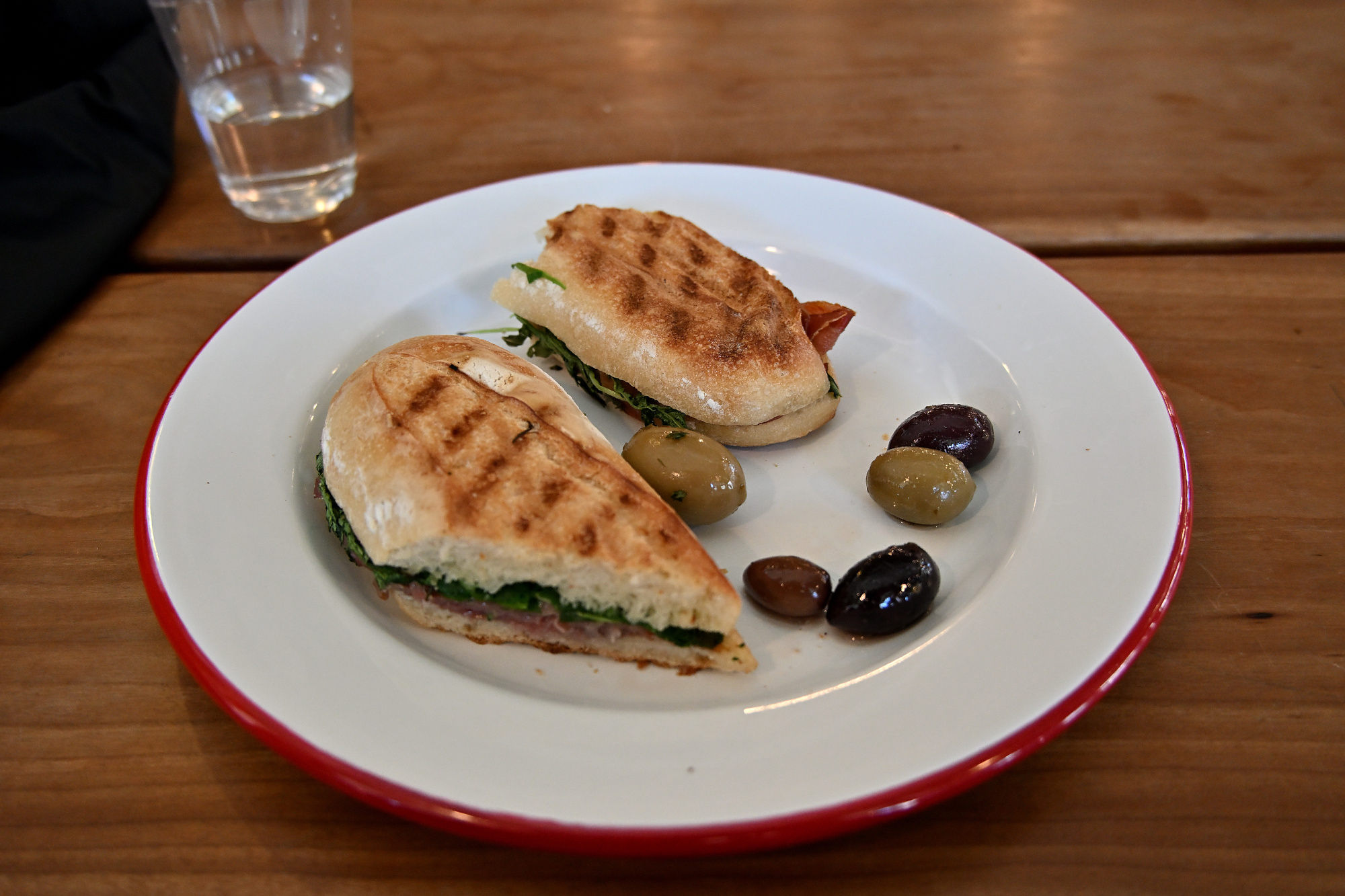
A small plate taking itself exactly as seriously as an Italian deli masterpiece should.
1/250s f/4 ISO 1100 18-140mm f/3,5-6,3 VR f=22mm/33mm
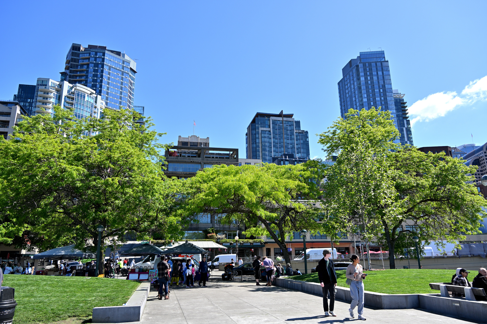
Outside for a moment, Pike Place remembers it has a sky.
Green space, blue sky, and the rare Seattle feeling that the weather is on your side.
1/320s f/6,3 ISO 100/21° 18-140mm f/3,5-6,3 VR f=18mm/27mm
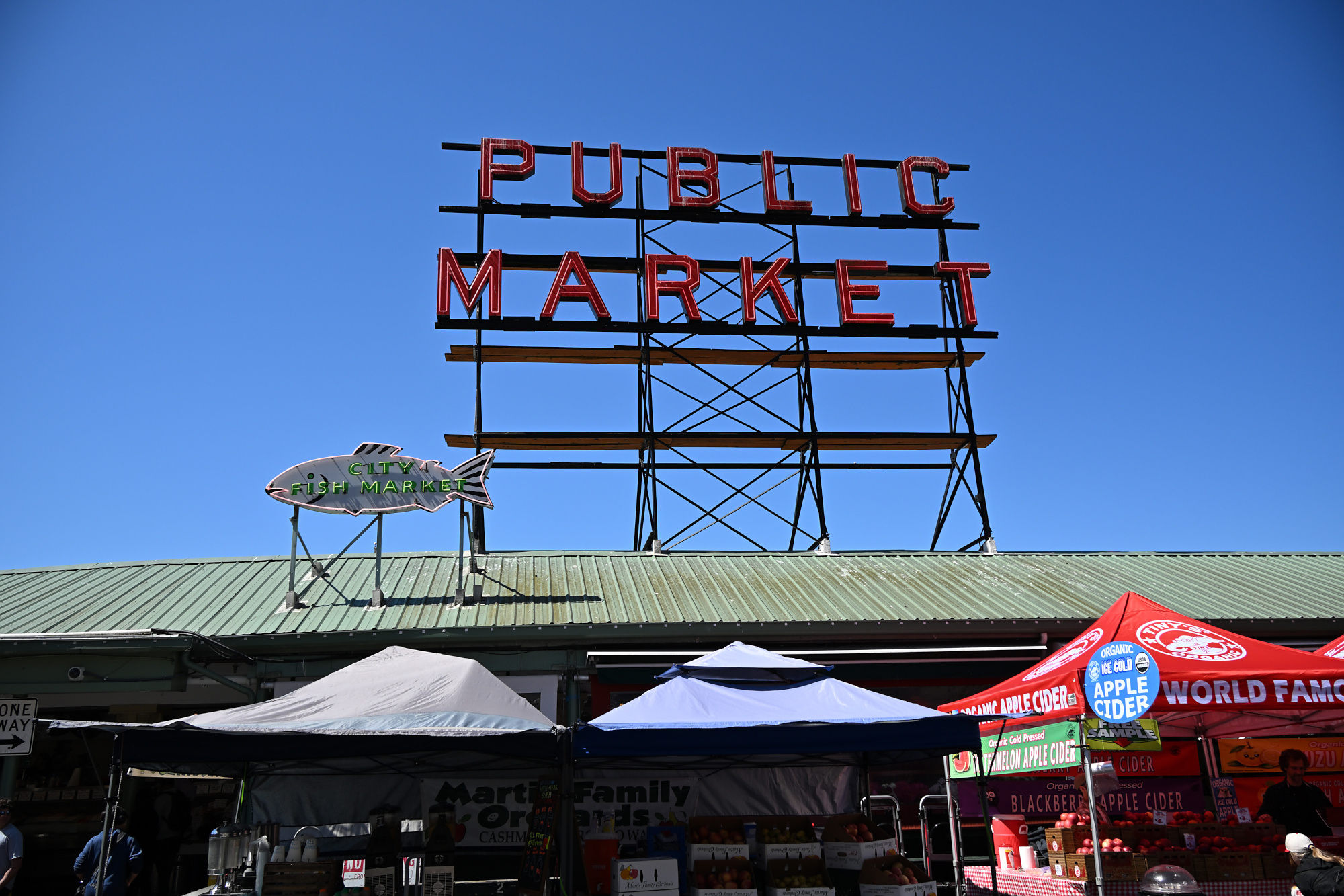
A second sign rises above the hall, making sure nobody forgets where they are.
1/400s f/7,1 ISO 100/21° 18-140mm f/3,5-6,3 VR f=18mm/27mm
At the fish counter, Pike Place makes its case for the best seafood in the Pacific Northwest.
A fish shop corner doing several jobs at once, with no visible management structure.
1/160s f/3,5 ISO 400/27° 18-140mm f/3,5-6,3 VR f=18mm/27mm
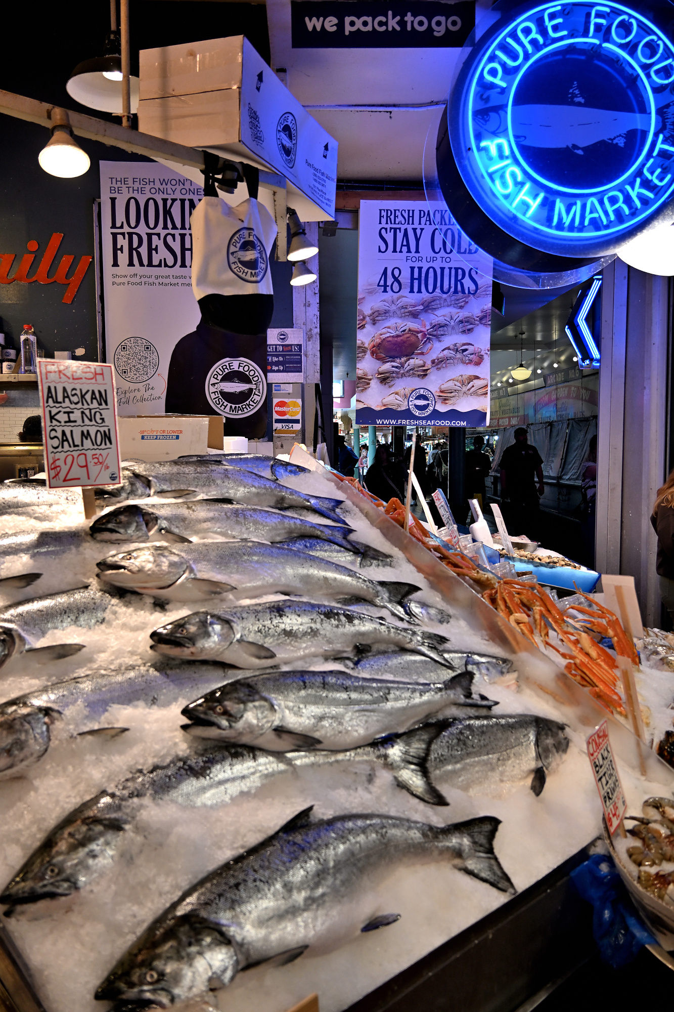
Blue signage, bright counters, and the clear sense that nobody here is under-selling the fish.
1/125s f/3,5 ISO 450 18-140mm f/3,5-6,3 VR f=18mm/27mm
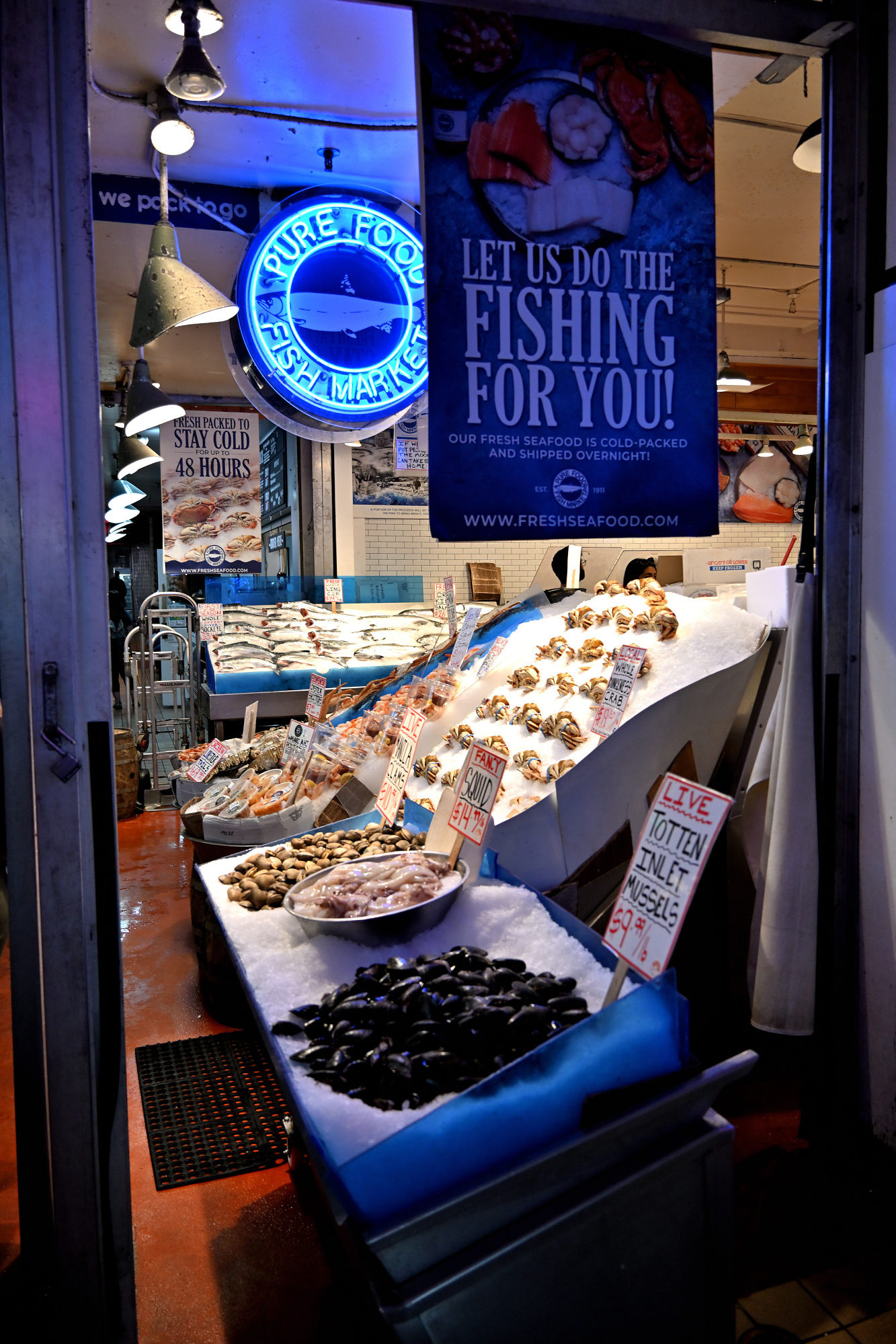
The display is so orderly that the fish almost look like they have appointments.
1/125s f/4 ISO 500/28° 18-140mm f/3,5-6,3 VR f=32mm/48mm
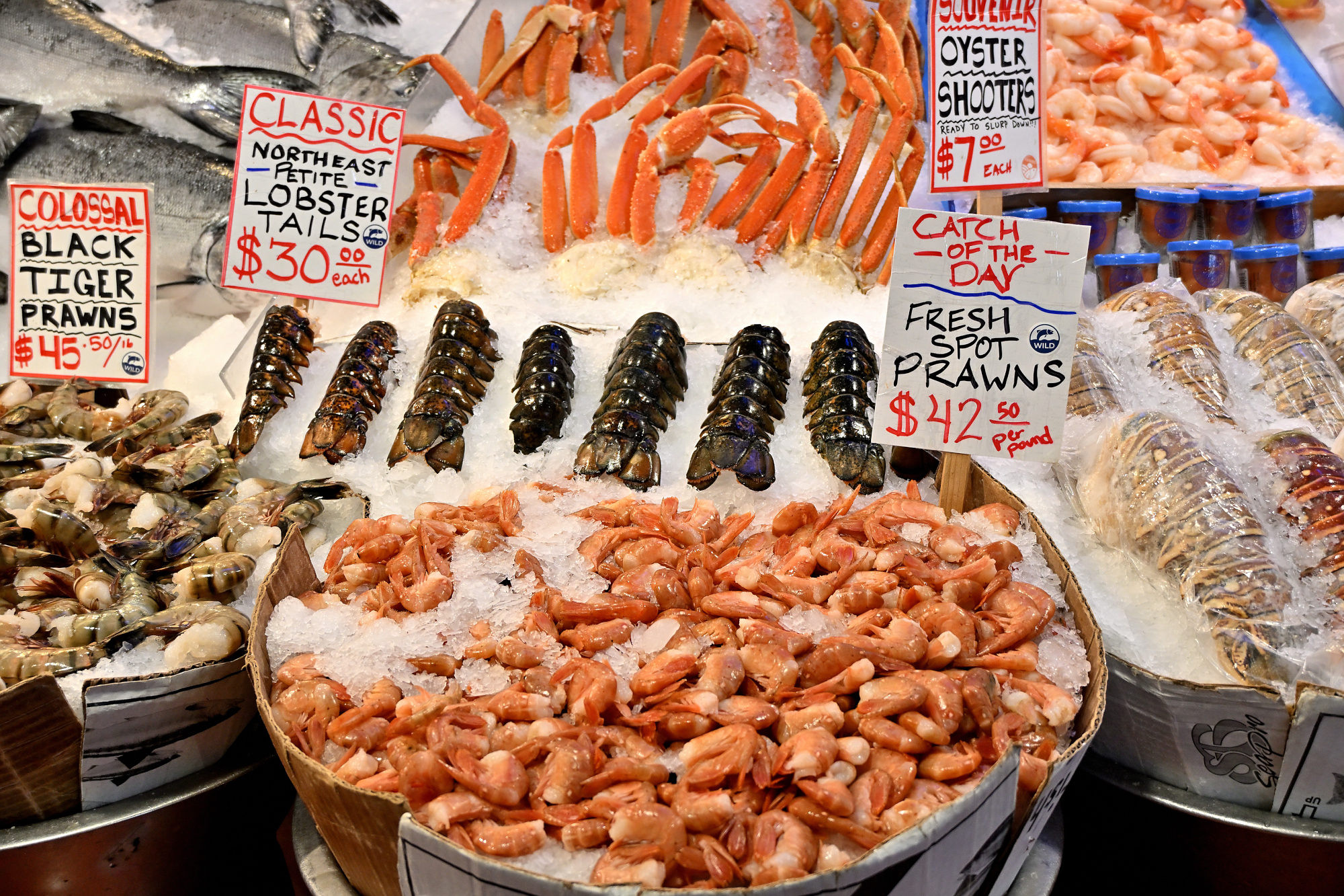
The counter is full, but nothing here seems in a hurry.
1/250s f/3,5 ISO 400/27° 18-140mm f/3,5-6,3 VR f=20mm/30mm
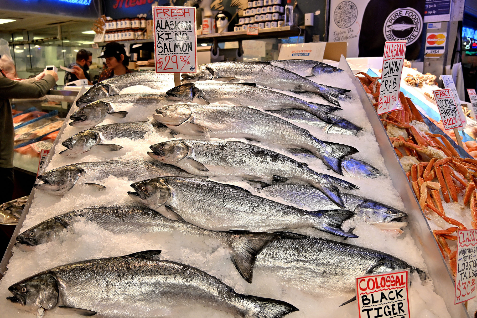
Here the whole display gets its moment, full but still holding itself together.
1/250s f/4 ISO 640/29° 18-140mm f/3,5-6,3 VR f=18mm/27mm
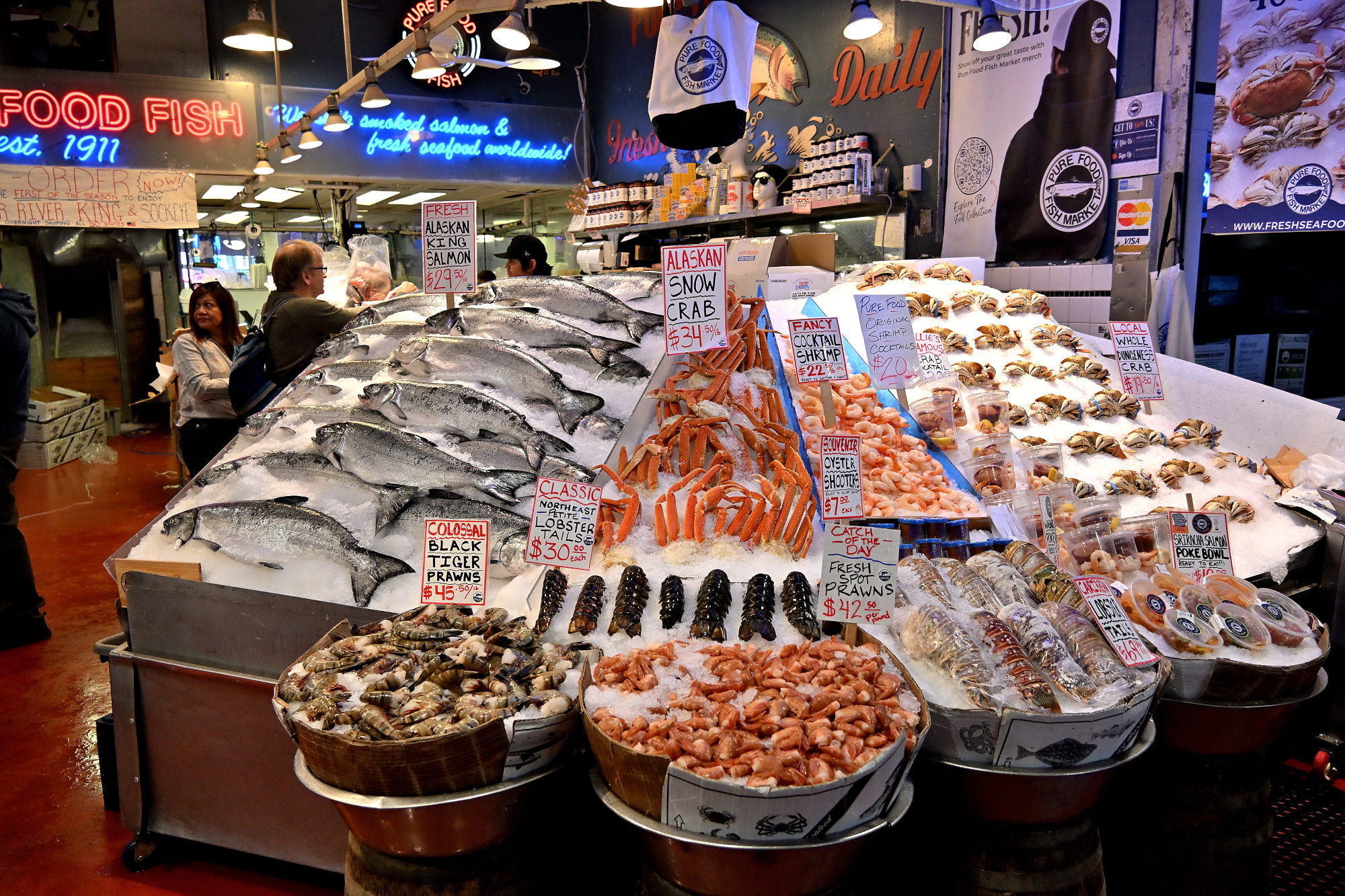
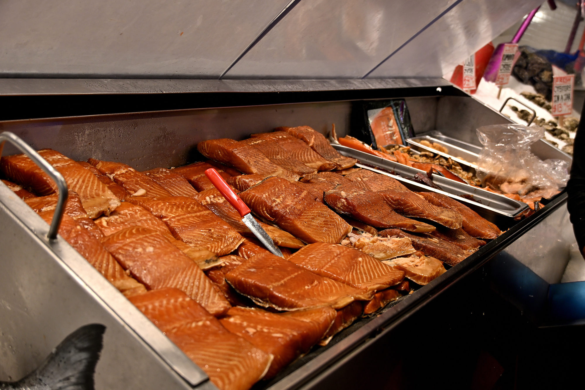
Smoked salmon in tidy rows, with the quiet confidence of being the best there is.
1/160s f/3,8 ISO 400/27° 18-140mm f/3,5-6,3 VR f=26mm/39mm
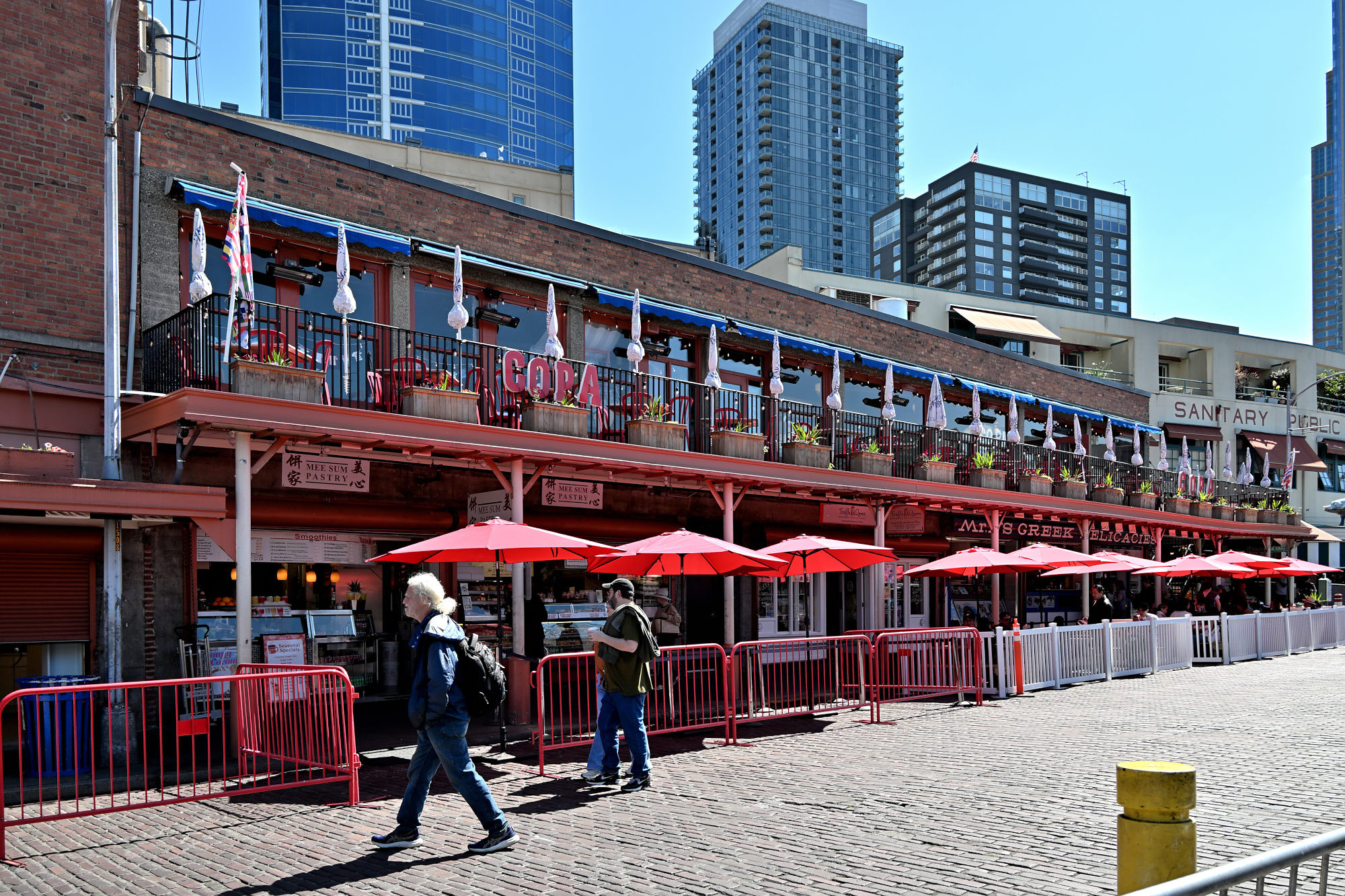
Away from the big fish counter, the market becomes a collection of smaller temptations and useful excuses.
Red umbrellas, brick, and just enough shade to make the street feel briefly organized. Hidden in plain sight is a weekend refrain that has been part of this corner for decades.
1/250s f/5,6 ISO 110 18-140mm f/3,5-6,3 VR f=18mm/27mm
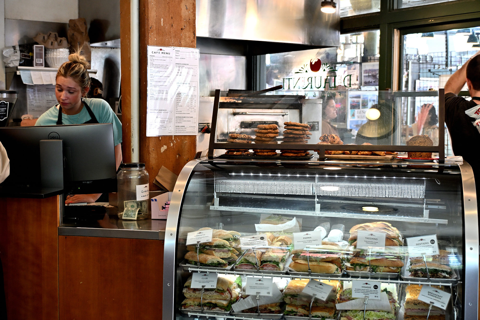
These Italian deli masterpieces wait here before their turn on the plate, already the best reason to come back.
1/125s f/4,2 ISO 900 18-140mm f/3,5-6,3 VR f=34mm/51mm
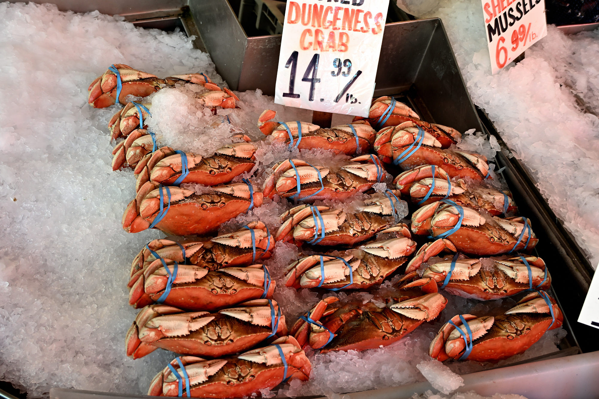
Another fish counter, because Pike Place apparently believes one seafood argument is not enough. The crabs look like they are waiting for a sponge, a starfish, and a squirrel to settle the business plan.
1/125s f/4 ISO 400/27° 18-140mm f/3,5-6,3 VR f=30mm/45mm
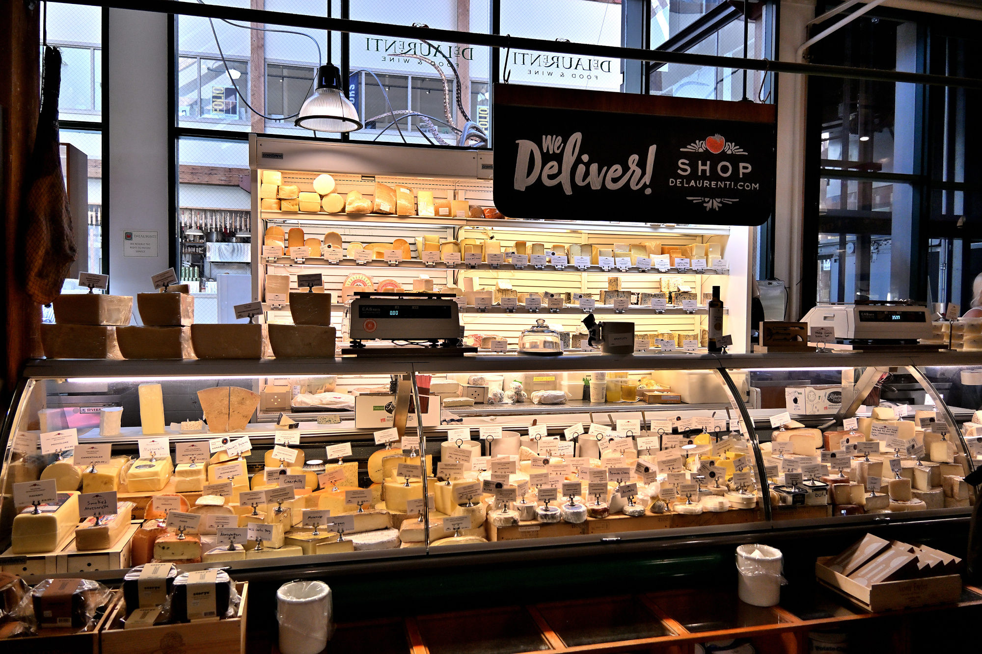
This is the kind of deli where leaving empty-handed starts to look like a personal failure.
1/250s f/4 ISO 400/27° 18-140mm f/3,5-6,3 VR f=18mm/27mm
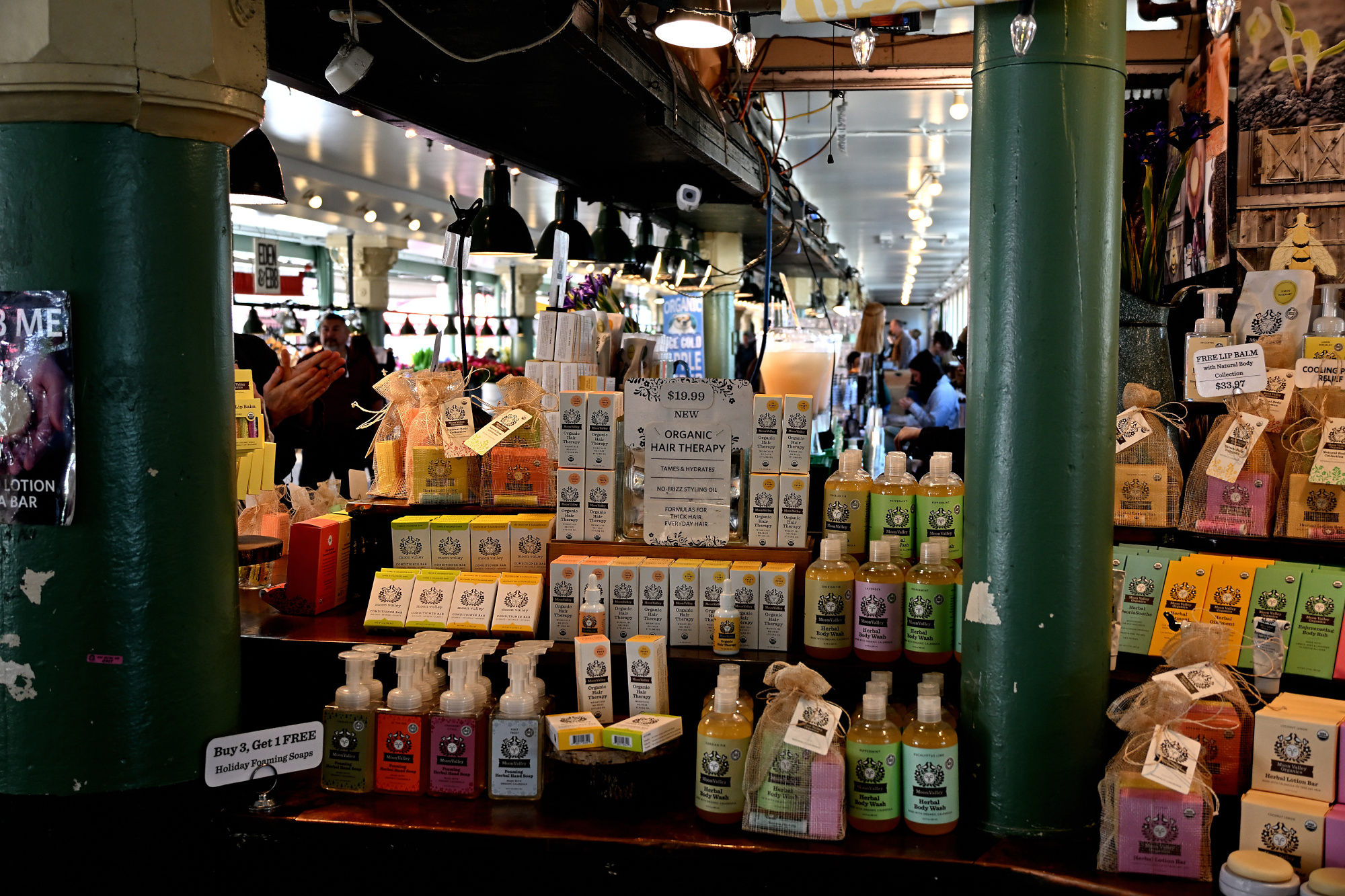
Soap on one side, honey on the other, and somehow the arrangement makes perfect market sense.
1/125s f/3,8 ISO 400/27° 18-140mm f/3,5-6,3 VR f=26mm/39mm
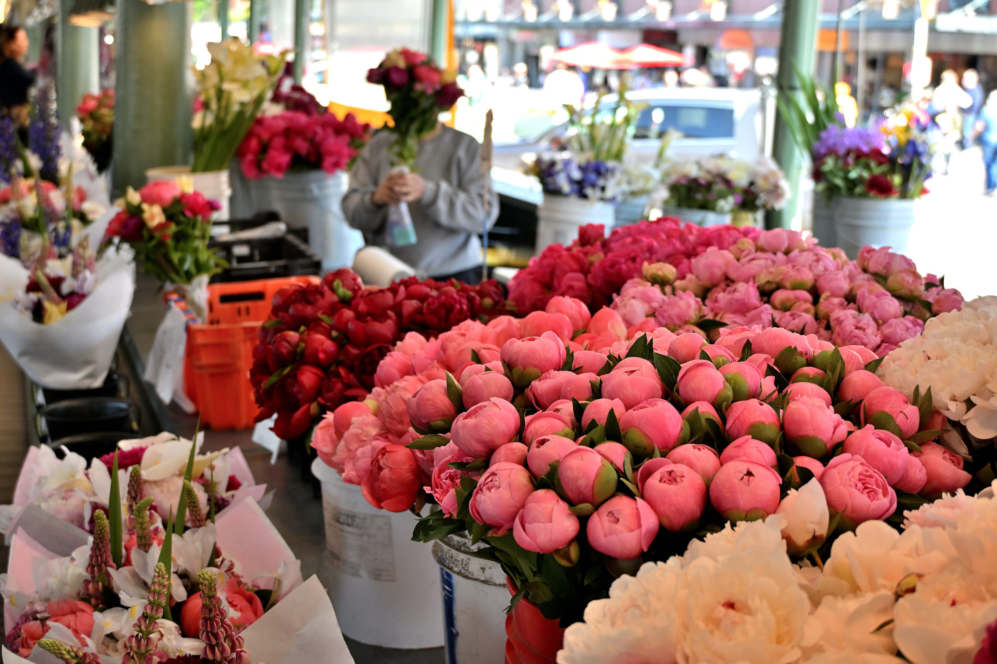
Every bouquet seems to be trying to outdo the one next to it.
1/200s f/4,2 ISO 400/27° 18-140mm f/3,5-6,3 VR f=34mm/51mm
The produce stand has enough options to make a simple decision feel optimistic.
1/125s f/3,5 ISO 1250/32° 18-140mm f/3,5-6,3 VR f=18mm/27mm
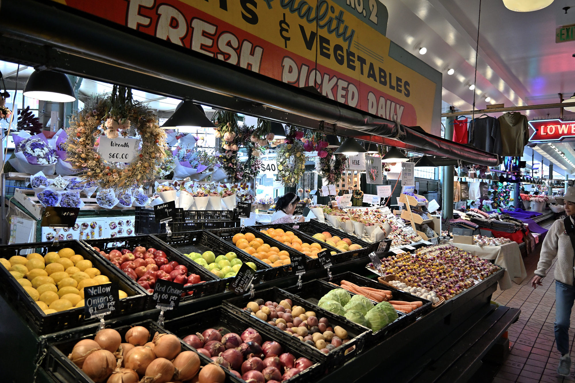
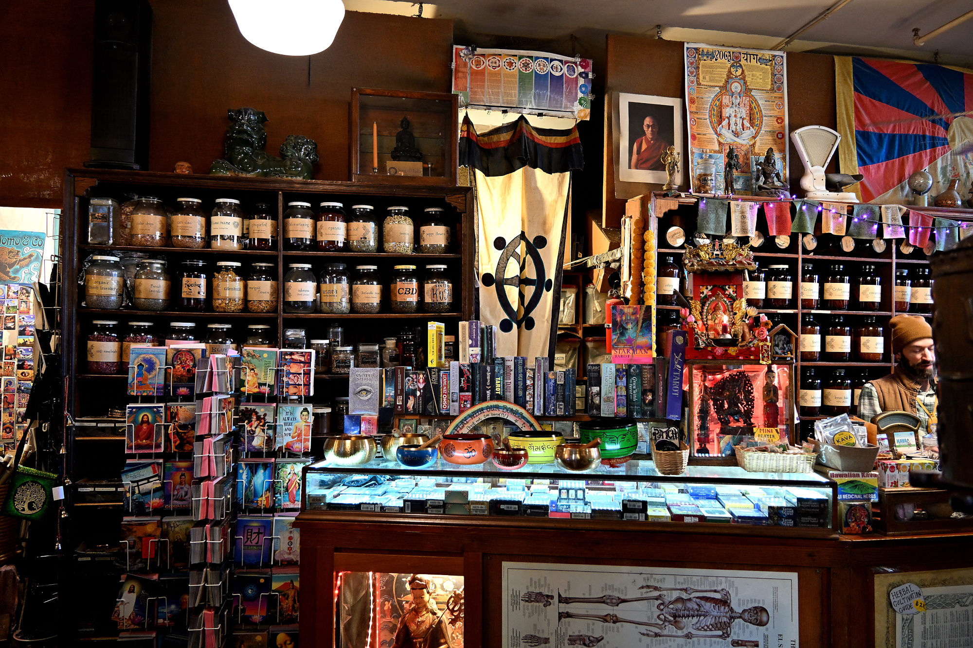
The shelves offer several small mysteries, most of them sealed in jars.
1/30s f/4 ISO 1100 18-140mm f/3,5-6,3 VR f=18mm/27mm
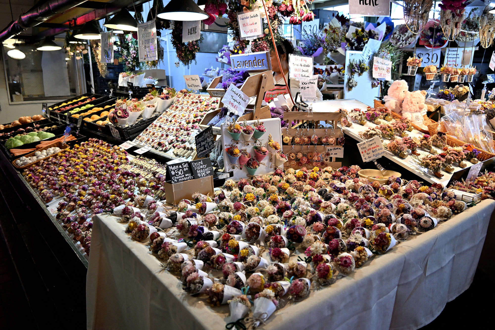
Dried flowers, making a quiet case for being just as beautiful.
1/125s f/3,5 ISO 800/30° 18-140mm f/3,5-6,3 VR f=18mm/27mm
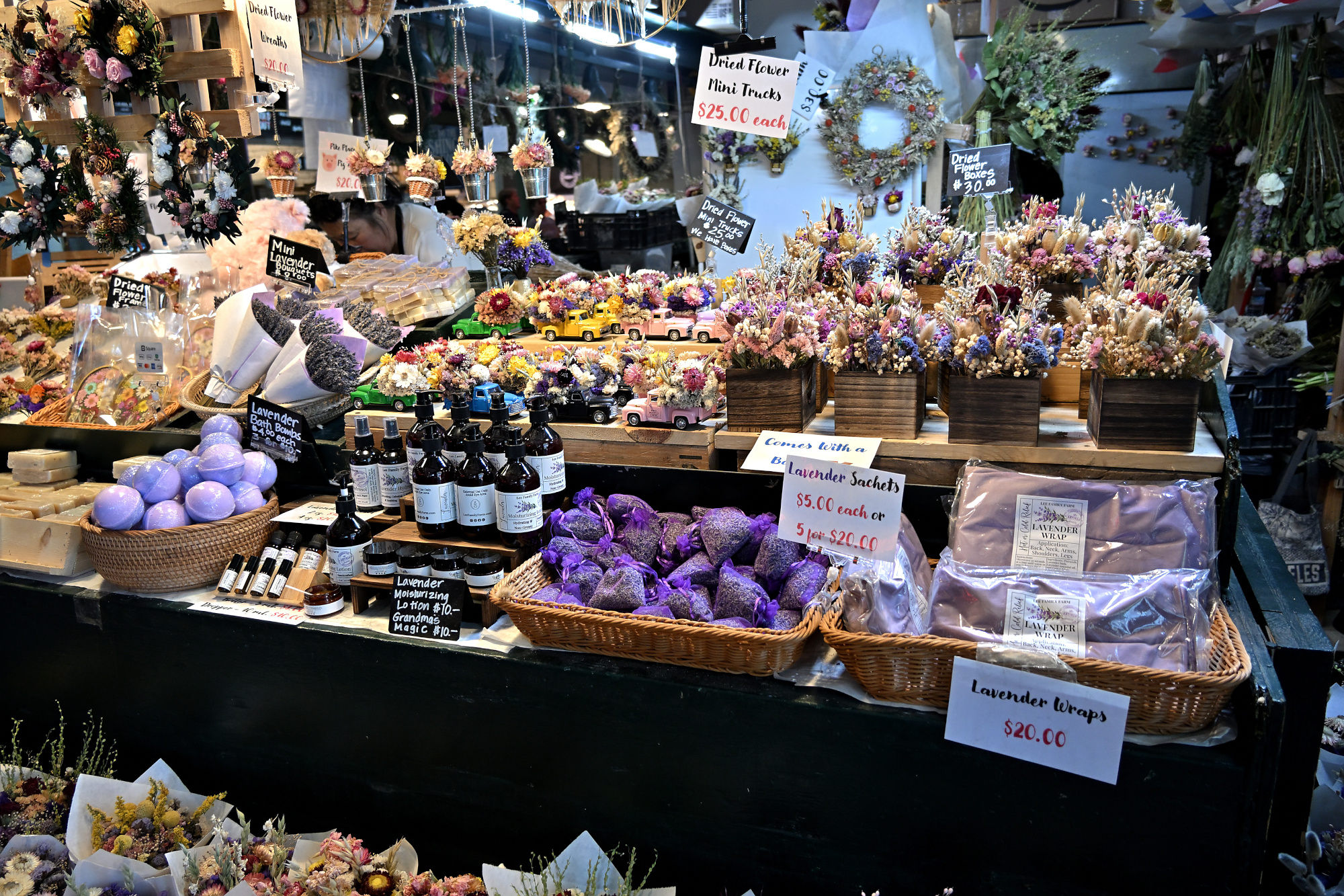
The dried bouquets keep making their quiet case.
1/125s f/3,5 ISO 800/30° 18-140mm f/3,5-6,3 VR f=18mm/27mm
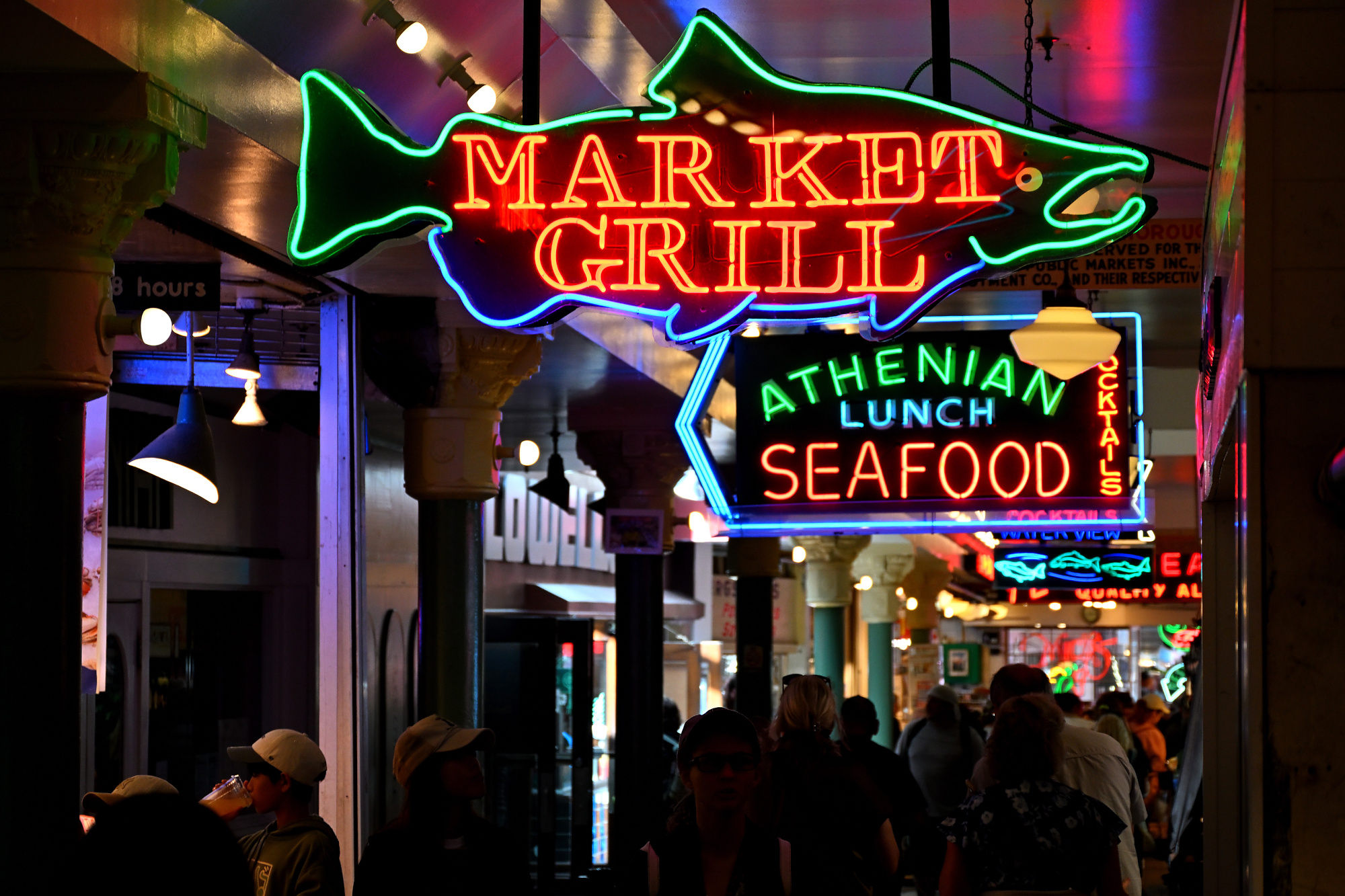
The neon fish sign has no interest in being subtle, which is probably for the best.
1/125s f/5,3 ISO 720 18-140mm f/3,5-6,3 VR f=77mm/115mm
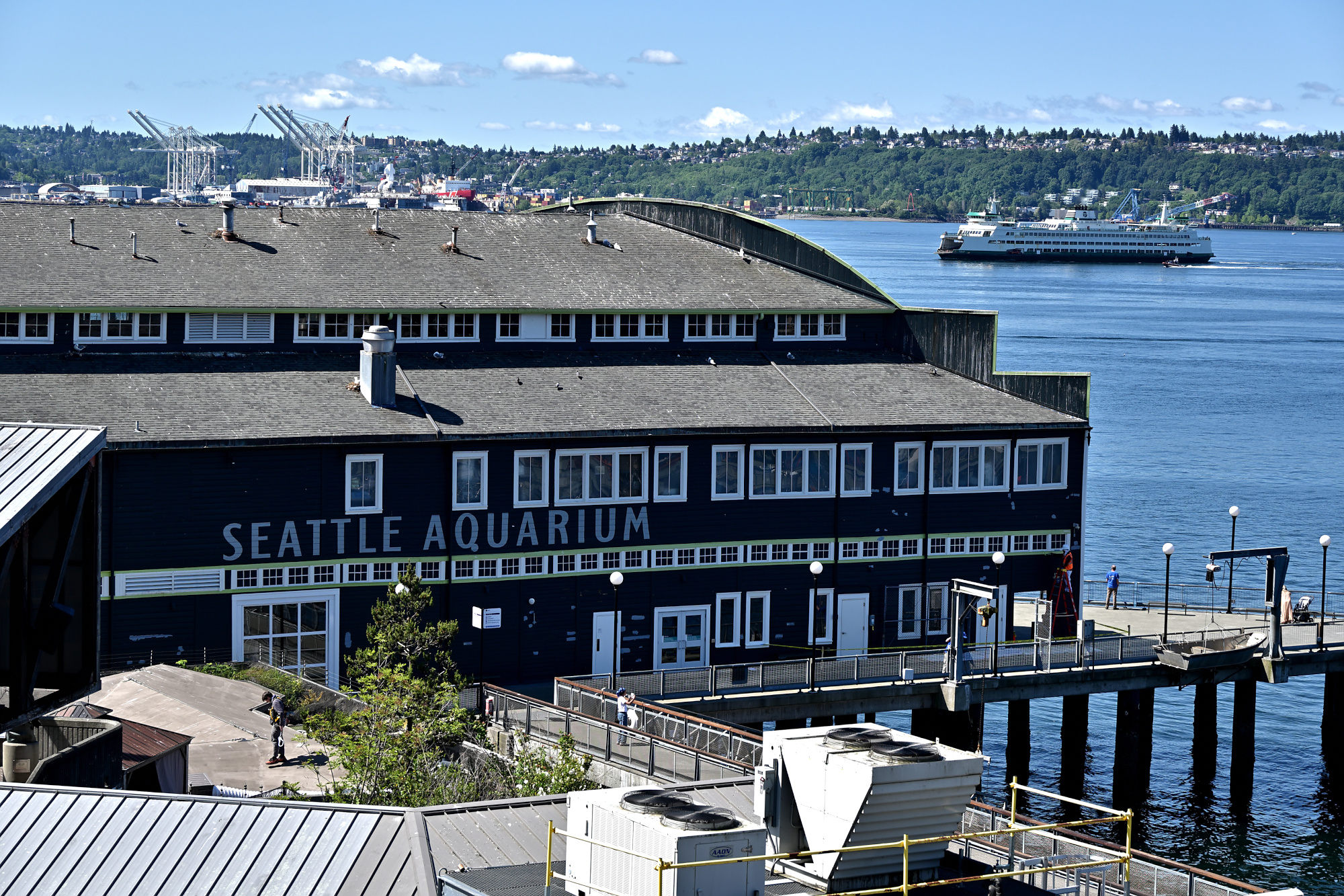
Eventually Pike Place opens back out toward streets, water, and light.
The Seattle Aquarium keeps watch over Puget Sound.
1/250s f/5,6 ISO 100/21° 18-140mm f/3,5-6,3 VR f=48mm/72mm
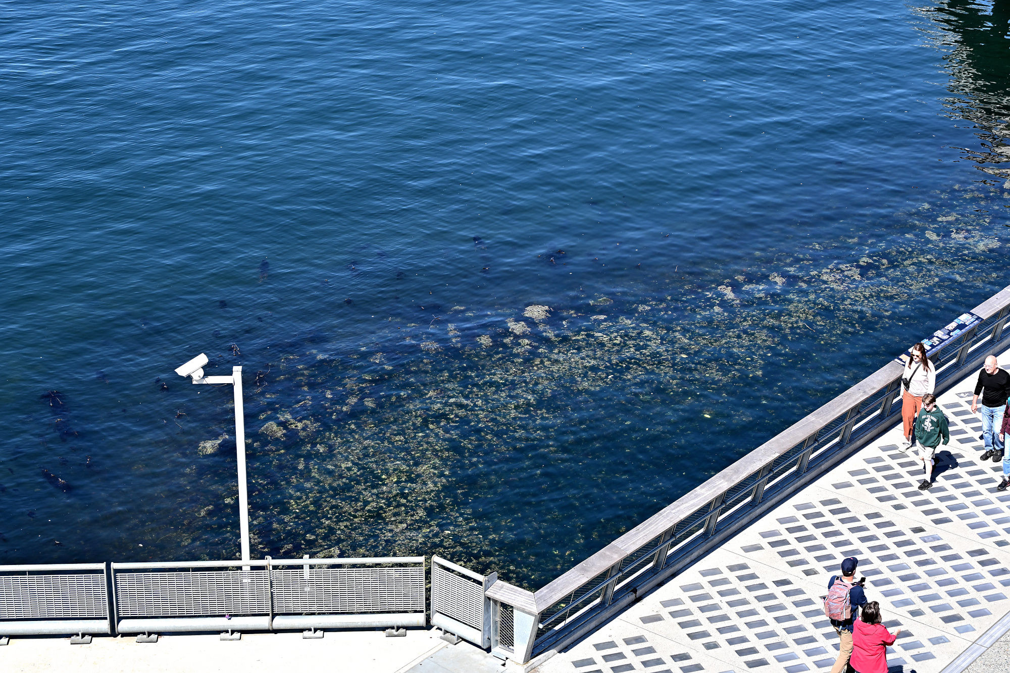
The waterfront drops away below, because Seattle likes its views with a little vertical planning.
1/250s f/5,6 ISO 125/22° 18-140mm f/3,5-6,3 VR f=51mm/76mm
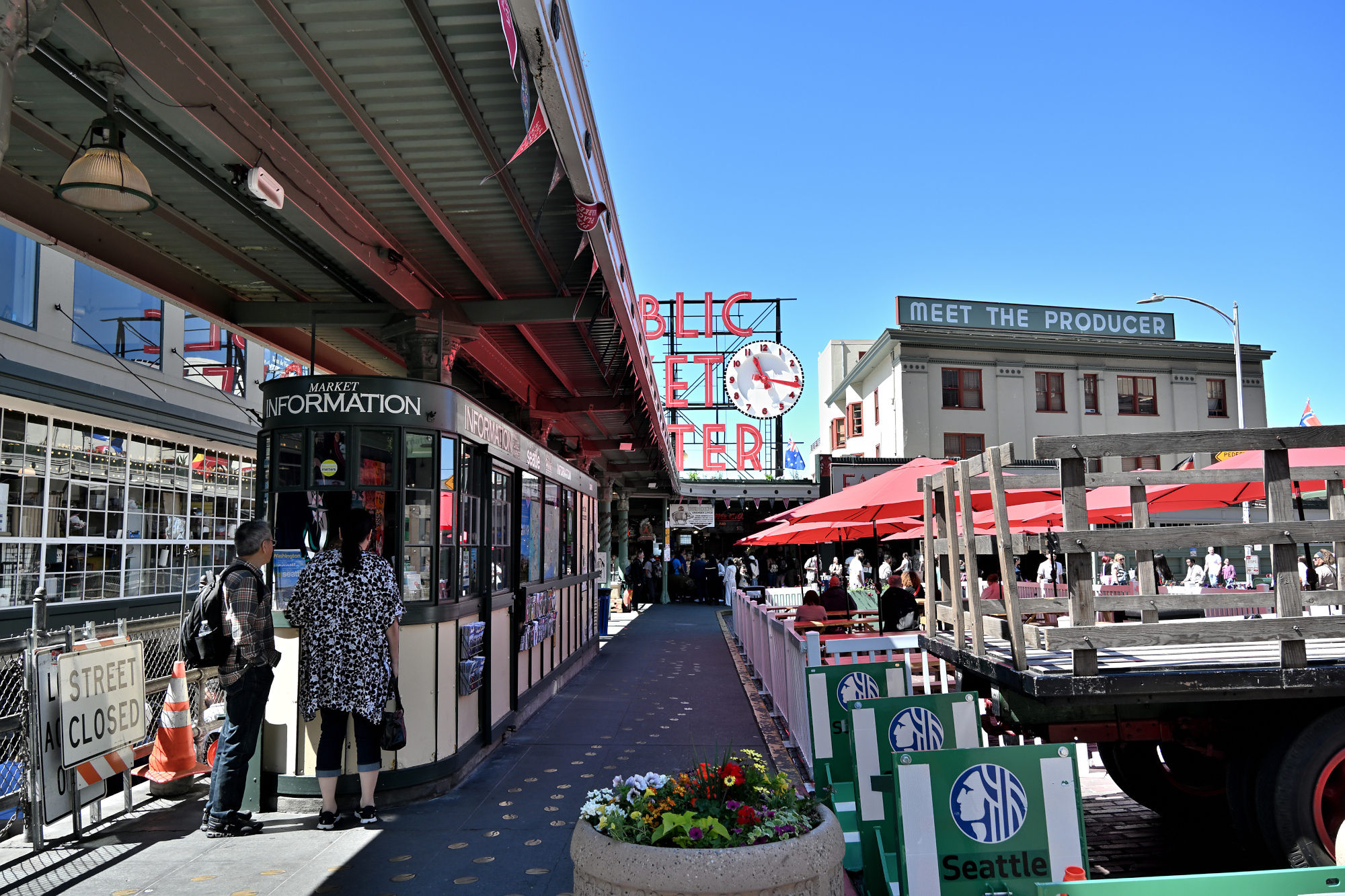
Back at the main market square, Pike Place does not need the whole sign to be recognizable.
1/250s f/5,6 ISO 200/24° 18-140mm f/3,5-6,3 VR f=18mm/27mm
Down by the water, the city finally leaves a little space between things.
1/500s f/8 ISO 100/21° 18-140mm f/3,5-6,3 VR f=85mm/127mm
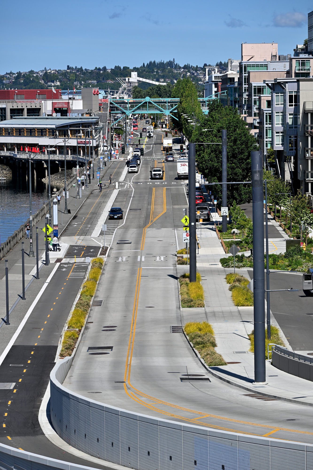
Green, blue, and concrete doing their best to make infrastructure look relaxed.
1/320s f/6,3 ISO 100/21° 18-140mm f/3,5-6,3 VR f=31mm/47mm
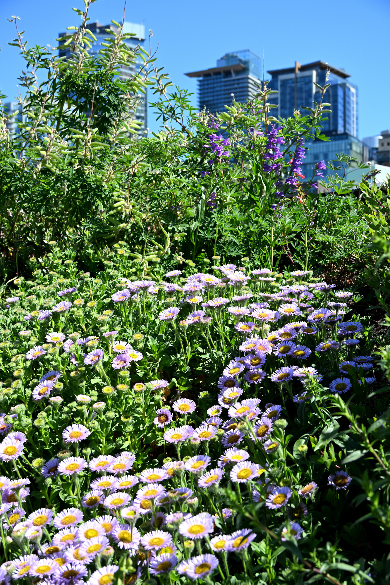
One last stretch of water, because some endings are better when they keep things simple.
1/500s f/11 ISO 200/24° 18-140mm f/3,5-6,3 VR f=130mm/195mm
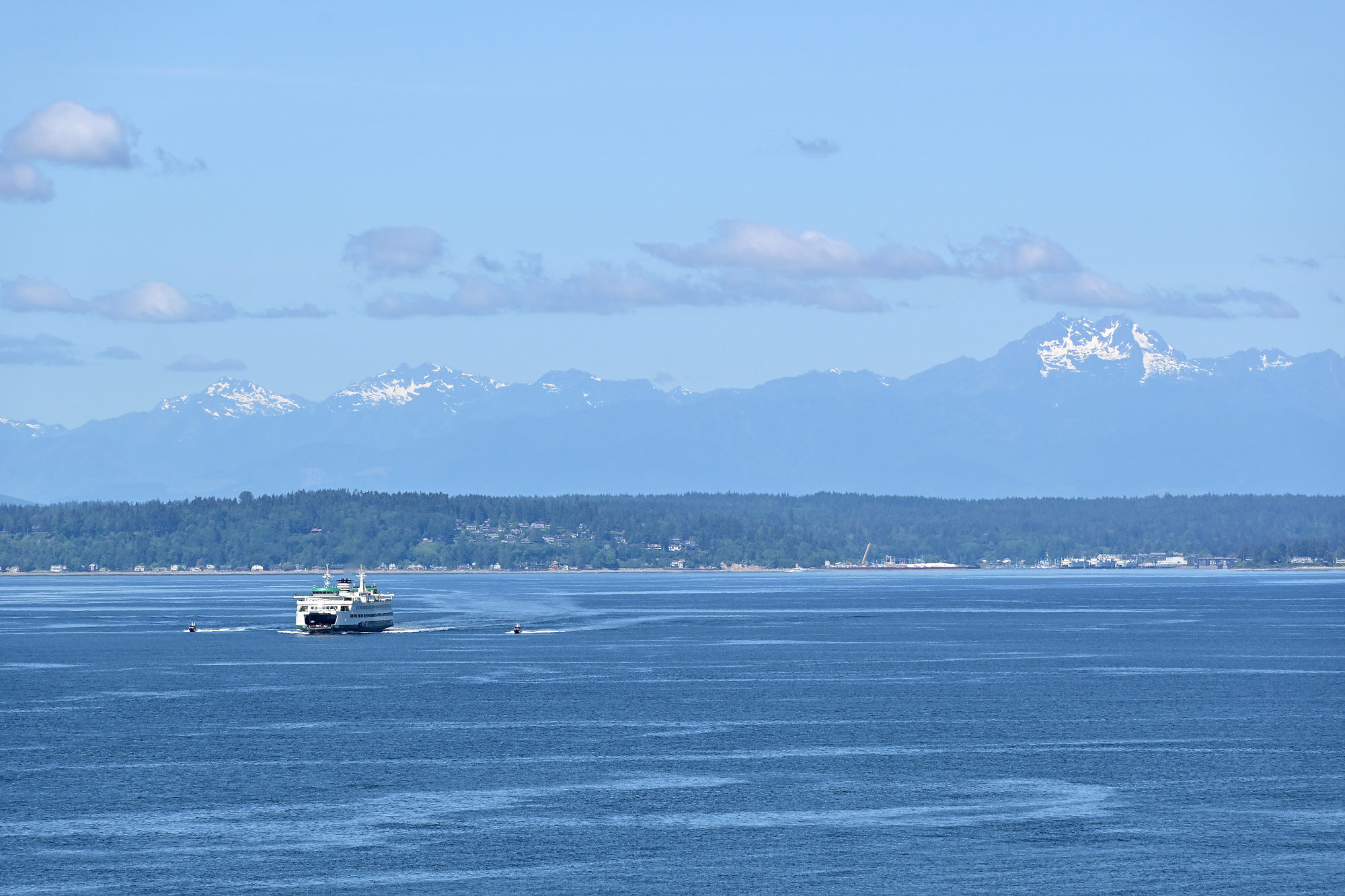
Taken with my Nikon Z50II.